Rebuilding ESP32-fluid-simulation: an outline of the sim task (Part 3)
Okay, I wondered if I should have led this series with the physics, but I think saving it for last was the right call. As I was writing about the FreeRTOS tasks involved and their communication and the touch and render tasks specifically, I started to think about how I could write about this with the detail and approachability it deserves.
To start, I’ll be honest: I’m not presenting anything groundbreaking here. In 1999, Jos Stam introduced a simple and fast form of fluid simulation in his conference paper called “Stable Fluids”, and in 2003, he published a straightforward version of it in “Realtime Fluid Dynamics for Games”. Many people have written guides to “fluid simulation” that have been specifically based on these two papers since. Two key examples to me: a chapter of NVIDIA’s GPU Gems and a blog post by Jamie Wong. To be pendantic, I find now that the current field of fluid simulation is much, much larger than what any of these references imply. Still, these were the guides I followed when I first wrote ESP32-fluid-simulation. In both was Stam’s technique, and between everything I just linked to, you could probably write your own implementation of it eventually.
That said, between then and when I rewrote it recently, I picked up some background knowledge that proved incredibly useful. I’m not saying here that I became an expert on fluid sims—I can’t advise you on designing a new technique from scratch. Rather, if I had known it back then, I wouldn’t have made nearly as many wrong turns. It turns out that implementing Stam’s technique gets easier when you understand the whats of the operations he would have you write, if not the whys.
Review: Vector fields and scalar fields
If you recall any vector calculus, then “vector fields” and “scalar fields” may be an obvious concept to you already, but if not, we can start with the fact that they’re a part of the foundation of fluid dynamics. For now, I’ll review what they are. However, I highly recommend picking up a total understanding of vector calculus somewhere else before looking at any fluid sim techniques besides Stam’s. In fact, perhaps fluid simulations make just the right concrete example to keep in mind while learning!
Anyway, let’s sketch out what vector fields and scalar fields are, and hopefully, the picture is filled in as you keep reading this article. The ordinary idea of a mathematical function is a thing that outputs a number when given a number input. Vector fields and scalar fields are functions—though of different kinds.
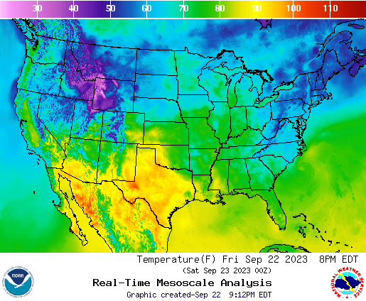
Consider a flat, two-dimensional space, and then consider a function that outputs a number when given a location in this space as the input. Furthermore, this location can be expressed as a pair of numbers if we used a coordinate system (three if we worked in three dimensions, and we could, but we won’t here). A concrete example of this would be a function of a location that gives the temperature there—the location being written as the latitude and longitude on the map. It’s 48 degrees Fahrenheit in Arkhangelsk and 84 degrees in Singapore. Considering that Arkangelsk can be found at 64.5°N, 40.5°E and Singapore at 1.2°N, 103.8°E, we can define a temperature function that gives $T(64.5, 40.5) = 48$ and $T(1.2, 103.8) = 89$. We can call it a temperature field, but more generally, it’s a “scalar field”. It’s a scalar-valued function of the location, possibly written as $f(x, y)$.
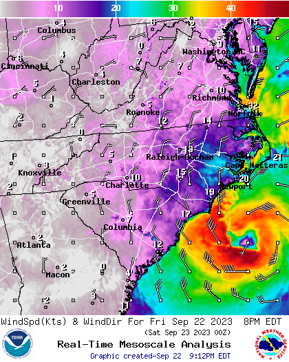
Now on the other hand, a “vector-valued function” is any function that outputs a vector, and a vector-valued function of a location is a “vector field”! A concrete example of this would be a wind velocity field. For any location, such a field would give how fast the wind there blows and the direction in which it goes, and it would be given as the magnitude and direction of a single vector. Like for scalar fields, we could possibly write them as $\bold{f}(x, y)$, the boldface font meaning that we have a vector output.
That said, though functions of location they are, written like one they are really not. Rather, the dependence on location is assumed, and then $f(x, y)$ and $\bold{f}(x, y)$ are just written as $f$ and $\bold{f}$ instead. Another thing to keep in mind: coordinates are just a pair of numbers, but we can also think of them as a single coordinate vector. Though we may never actually draw that arrow, the interchangeability is relevant. For example, I briefly talked in the previous post about the similarity between a velocity vector and a change in the coordinate vector over a finite period of time.
First, it would be helpful to picture what we want to simulate. The input and output are the touch and screen of a touchscreen, and the user dragging around the stylus on it should stir around the fluid on display. The physical scenario this should match is if someone stuck their arm into a bed of dyed water and then stirred it around. In such a scenario, the color would be determined by the concentration of the dye, but the dye itself moves! To capture this physical behavior with a computer simulation, we can start by describing it with a mathematical model.
In Stam’s “Real-time Fluid Dynamics for Games”, he wanted to capture smoke rising from a cigarette and being blown around by air currents. To do so, he ascribed a velocity field (a vector field) and a smoke density field (a scalar field) to the air. But that was it for his model: everything else about it he threw out. In the same way, we can reduce the bed of water to just a velocity field and a dye concentration field.
Now, what was the relationship between these two fields? Stam wrote that the density field undergoes “advection” by the velocity field. That’s the process of fluid carrying around (smoke particles, dye, or anything in general), and this happens everywhere. He also wrote that it undergoes “diffusion”, which is the spontaneous spreading of a thing in a fluid from areas of higher density without being carried by the velocity. He provided an “advection-diffusion” equation that captures both, and it’s a “partial differential equation”.
Review: Partial derivatives and the differential operators
Just like how we can take the derivative of your ordinary function, we can take a differential operator of a field. However, these differential operators don’t just mean the slope of a tangent line, but rather they each represent a different way the field changes over a change in location. The critical ones to understand here are the “divergence” and the “gradient”, but the “Laplacian” is also worth touching on. (A formal vector calculus course would also cover the “curl”, the identities, and the associated theorems.)
First of all, differential operators are constructed from the “partial derivatives”. These are the derivatives you already know, but we strictly take them with respect to one of the components while holding the others constant. The reason? Formally, your ordinary derivative is the limit of the change in your ordinary function $f(x)$ over the change in the input $x$ as that change in the input approaches zero.
\[\frac{df}{dx} = \lim_{\Delta x \to 0} \frac{f(x+\Delta x) - f(x)}{\Delta x}\]However, in the case of fields, by doing this to only one of the components of the location coordinate, the partial derivative just formally means the change in the field $f(x, y)$ over the change in that component. Keeping the other components constant is naturally a part of measuring this change. In two dimensions, fields can have a partial derivative with respect to $x$ or one with respect to $y$. Then, $y$ or $x$ respectively is held constant.
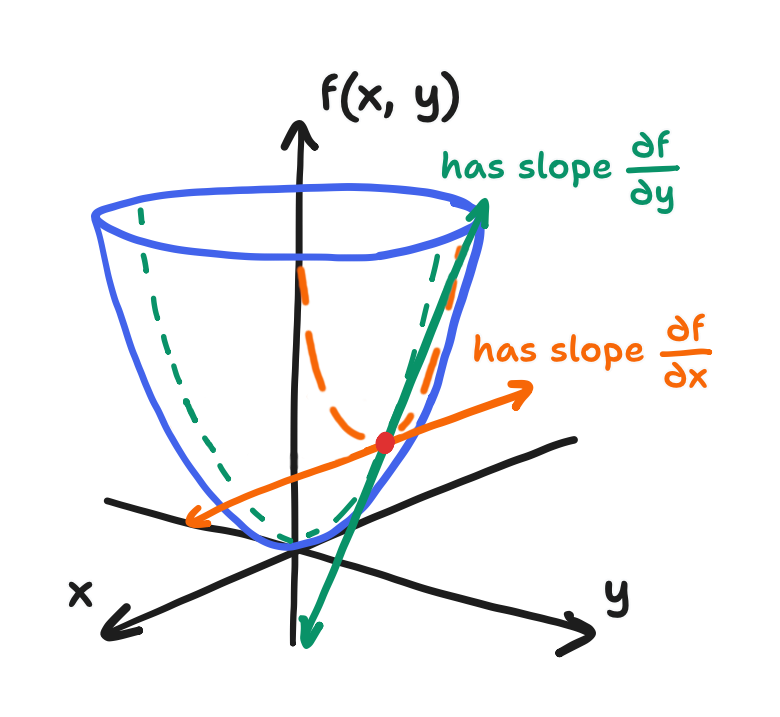
\[\frac{\partial f}{\partial x} = \lim_{\Delta x \to 0} \frac{f(x + \Delta x, y) - f(x, y)}{\Delta x}\] \[\frac{\partial f}{\partial y} = \lim_{\Delta y \to 0} \frac{f(x, y + \Delta y) - f(x, y)}{\Delta y}\]A good example would actually be to perform a derivation. Given the function $f(x, y) = x^2 + 2xy + y^2$ as a field, let’s find the partial derivative with respect to $x$.
\[\begin{align*} \frac{\partial}{\partial x}(x^2 + 2xy + y^2) & = 2x + 2y + 0 \\ & \boxed{ = 2x + 2y } \end{align*}\]Notice that—because $y$ is taken as a constant—$y^2$ drops out and $2xy$ is treated as an $x$-term with a coefficient of $2y$. And finally, to expand on this a bit with a geometric picture, we know that the derivative is the slope of the tangent line, but to be exact, it’s the line tangent to the curve of $f(x)$ at the point $(x, f(x))$. The partial derivative is still the slope of a line that is tangent to the surface of the field at the point $(x, y, f(x, y))$, but it is also strictly running in the $x$-direction for $\partial/\partial x$ or in the $y$-direction for $\partial/\partial y$. Technically, infinitely many lines satisfy the conditions of being tangent to the surface at that point, and these lines form a tangent plane, but we only concern ourselves with the two.
That aside, taking a partial derivative with respect to some single component is not as useful as taking every partial derivative with respect to each component. This set is written like a vector of sorts (though a vector it is not) called the “del operator”. For two dimensions, that is
\[\nabla \equiv \begin{bmatrix} \displaystyle \frac{\partial}{\partial x} \\[1em] \displaystyle \frac{\partial}{\partial y} \end{bmatrix}\]The constructions out of this set that we call the differential operators can absolutely be written without using the del operator, but you’d usually see that they are.
The “gradient” is the simplest construction: line up each and every partial derivative of a scalar field into a vector. Keeping in mind here that the partial derivative of a field (like $x^2+2xy+y^2$) is actually yet another function of the location (like $x^2 + 2y$), a vector composed of these will itself vary by the location. The gradient of a scalar field is a vector field! We can get to exactly how the gradient gets applied to our fluid sim later, but one useful fact to picture here is that it can be shown that the gradient always happens to point in the direction of steepest ascent in the scalar field. Walking in the direction of the gradient of the temperature field, for example, would warm you up the fastest!
\[\nabla f = \begin{bmatrix} \displaystyle \frac{\partial f}{\partial x} \\[1em] \displaystyle \frac{\partial f}{\partial y} \end{bmatrix}\]Using the del operator, it looks kind of like scalar multiplication from the right.
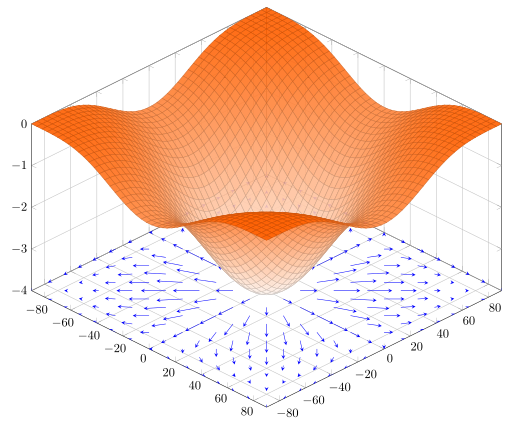
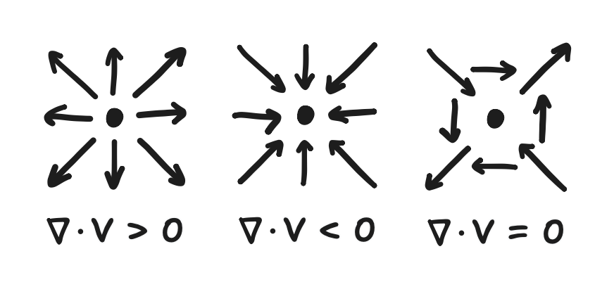
And remember, the gradient is just one shockingly meaningful operator that we can construct from the partial derivatives, which were just slopes of tangent lines! The “divergence” is a slightly more complicated construction: if we write out a vector field using its components
\[\bold{f}(x, y) = \begin{bmatrix} f_x(x, y) \\ f_y(x, y) \end{bmatrix}\]then we can take the partial derivative of each component with respect to its associated component of the coordinates (that’s $f_x$ to $\partial/\partial x$ and $f_y$ to $\partial/\partial y$) and then add them up. We should be able to recognize here that the divergence of a vector field is a scalar field. And what is the meaning of this scalar field? For now, it can be imagined as the degree to which the vectors surrounding an input location are pointing away from it, though Gauss’s theorem expresses this more formally (a bit out-of-scope for now).
\[\nabla \cdot \bold{f} = \frac{\partial f_x}{\partial x} + \frac{\partial f_y}{\partial y}\]Using the del operator, it looks kind of like a dot product.
Finally, the “Laplacian” is actually the divergence of the gradient of a scalar field, and this ultimately means that it’s also a scalar field! It is also the sum of the second-order partial derivatives (besides the mixed ones, but that’s totally out-of-scope).
\[\nabla^2 f \equiv \nabla \cdot (\nabla f) = \frac{\partial^2 f}{\partial x^2} + \frac{\partial^2 f}{\partial y^2}\]Using the del operator, some take the liberty of expressing this composition as a single $\nabla^2$ operator.
There is also the extension of the Laplacian onto vector fields, but it really is just the Laplacian on each component.
\[\nabla^2 \bold{f} = \begin{bmatrix} \nabla^2 f_x \\ \nabla^2 f_y \end{bmatrix}\]The gradient, divergence, and Laplacian are all the differential operators that are relevant here, and hopefully these will become more concrete to you as we use them from here on to describe Stam’s fluid sim technique. However, I’d again recommend formally learning vector calculus if you’d like to look at other techniques.
A “partial differential equation” is kind of like a system of linear equations in this context. Here, they still relate known and unknown variables, and they still have a solution which is the value of the unknowns. However, these “values” are entire fields, not just numbers! Given this, partial differential equations also involve the differential operators of these field-valued variables.
The advection-diffusion equation that Stam provides is a simple example of one: advection and diffusion are independent terms, and their sum is exactly how the density field evolves over time. It is
\[\frac{\partial \rho}{\partial t} = -(\bold{v} \cdot \nabla) \rho + \kappa \nabla^2 \rho + S\]where $\rho$ is the density field and $\bold{v}$ is the velocity field. $-(\bold{v} \cdot \nabla) \rho$ is the advection term, and $\kappa \nabla^2 \rho$ is the diffusion term—$\kappa$ being a constant for us to control the strength of the diffusion. $S$ is just a term that lets us add density (of smoke, or concentration of dye in our case) to the scene. Notice how this equation is a definition of $\partial \rho / \partial t$. It’s the partial derivative of the density field with respect to time, and it means that $\rho$ is a variable whose value is a function of location and time. However, it’s more useful for us to think of it equivalently as a field that evolves over time. An evolving density field is exactly what we want to show on the screen!
You may also notice that $(\bold{v} \cdot \nabla)$ is clearly some kind of construction from the partial derivatives because it uses the del operator $\nabla$. That is the “advection” operator. I’ve only seen it in fluid dynamics papers and yet still don’t totally understand it. Still, we’ll see how Stam treats it, but that’ll have to be in the next post.
All said though, where is the room in this model for the user’s input? Is the velocity field just a thing we get to set? (Right now, we have two unknowns, $\rho$ and $\bold{v}$, but one equation!) No, it’s more complicated than that: the way water and air move continues to change even after we stop stirring it. That leads to the missing piece to stirring digital water: we need a physical way to define $\partial \bold{v} / \partial t$ (a.k.a. the acceleration!) just like how $\partial \rho / \partial t$ was defined. That missing piece is the famous “Navier-Stokes equations”.
The “Navier-Stokes equations” are also partial differential equations. A definition of Navier-Stokes can be found in any fluid dynamics article, but the one Stam provided in “Stable Fluids” is the most directly relevant one.
\[\frac{\partial \bold{v}}{\partial t} = -(\bold{v} \cdot \nabla) \bold{v} - \frac{1}{\rho} \nabla p + \nu \nabla^2 \bold{v} + \bold{f}\] \[\nabla \cdot \bold{v} = 0\]The first one is a definition of $\partial \bold{v} / \partial t$. Here, $-(\bold{v} \cdot \nabla) \bold{v}$ and $\nu \nabla^2 \bold{v}$ represent advection and diffusion again, though these are also known as “convection” and acceleration due to “viscosity”, respectively. That is to say, the velocity is carried around and diffused just like how the smoke density was. The only difference is that the constant $\nu$ here is the “kinematic viscosity”, and it’s higher for fluids like honey and lower for fluids like water. That aside, $\bold{f}$ represents the acceleration due to external forces, and there is the place in our mathematical model where the user input would go!
On the other hand, $-\frac{1}{\rho} \nabla p$ is an interesting term—it’s not independent here. Let me try to explain. Typically, like in gasses, it is an acceleration due to a difference in pressure, and the negative of the gradient represents the tendency for fluids to flow from regions of high pressure to regions of low pressure. (Since the gradient points in the direction of steepest ascent, then going in the opposite direction gives the steepest descent.) The pressure differences are in turn driven by things like temperature. But that’s not what we’re talking about today!
As Stam had put it, “[t]he pressure and the velocity fields which appear in the Navier-Stokes equations are in fact related”. Ultimately, $-\frac{1}{\rho} \nabla p$ is used like a correction term to guarantee that the second equation holds. Whereas the first equation reads as a sum of processes that make up the acceleration, the second equation, $\nabla \cdot \bold{v} = 0$, reads like this: the divergence of the velocity field (which is a scalar field, rememeber!) is equal to zero everywhere. Even as a fluid evolves, this is a constraint that it must satisfy throughout, and it’s termed the “incompressibility constraint”.
The incompressibility constraint is said to be critical for it to look like water. Unfortunately, knowing what it is turns out to not be the same as knowing why it is. That’s beyond what I can comfortably explain, and there’s enough to explain in regards to how the pressure term is used to satisfy it. There’s quite a lot to say on that front, actually, so it’ll be another matter to cover in the next posts.
That aside, I’m going to adjust the equations while we’re here. Because the overall project was about simulating dye in water on an ESP32 and not smoke in air on a GPU, I didn’t use the entire equation. Anyway, this can be thought of as an exercise in finding what part of the physics can be ignored while still looking sorta-physical, I suppose. I really have to wash my hands of any assertions I’m making at this moment, for I am no expert in this field. With that said, I can confirm that deleting the diffusion term by letting $\kappa = 0$ doesn’t look so egregious. We also don’t have to add more dye, so we can delete $S$ while we’re at it. That actually just leaves the advection alone.
\[\frac{\partial \rho}{\partial t} = -(\bold{v} \cdot \nabla) \rho\]Furthermore, I also got away with letting $\nu = 0$, deleting that term and reducing the Navier-Stokes equations to the following.
\[\frac{\partial \bold{v}}{\partial t} = -(\bold{v} \cdot \nabla) \bold{v} - \frac{1}{\rho} \nabla p + \bold{f}\] \[\nabla \cdot \bold{v} = 0\]So ends this post. With the governing equations (advection-diffusion and Navier-Stokes), we’ve laid out the fundamental outline of Stam’s technique. We’ve also reviewed the relevant vector calculus, though no more than that. Though I didn’t have all the authority I needed to get the whys, we should be equipped to understand the whats. In the last parts, we’ll fill in the outline to get an end-to-end fluid simulation. If you’re still here before the next post comes out though, there’s always the ESP32-fluid-simulation source code on GitHub.