Rebuilding ESP32-fluid-simulation: the advection and force steps of the sim task (Part 4)
If you’ve read Part 2 and Part 3 already, then you’re as equipped to read this part as I can make you. You’ve already heard me mention that we should be passing in touch inputs, consisting of locations of velocities. You’ve also already heard that we’re getting out color arrays. Some mechanism should be turning the former into the latter, and it should be broadly inspired by the physics, which we had written out as partial differential equations. This post and the next post—the final ones—are about that mechanism. To be precise, this post covers everything but the pressure step, and the next will give it its own airtime.
With that said, if I miss anything, the references I used might be more helpful. That’s primarily the GPU Gems chapter and Jamie Wong’s blog post, but there’s also Stam’s “Realtime Fluid Dynamics for Games” and “Stable Fluids”.
Now, to tell you what I’m gonna tell you, a high-level overview is this:
- apply “semi-Lagrangian advection” to the velocities,
- apply the user’s input to the velocities,
- calculate the “divergence-free projection” of the velocities—here making use of the pressure term to do it—and finally,
- apply “semi-Lagrangian advection” to the density array with the updated velocities.
The process has four parts, and each part corresponds to a part of the physics. Let’s recall the partial differential equations that we ended up with in Part 3, that is:
\[\frac{\partial \rho}{\partial t} = - (\bold v \cdot \nabla) \rho\] \[\frac{\partial \bold v}{\partial t} = - (\bold v \cdot \nabla) \bold v - \frac{1}{\rho} \nabla p + \bold f\] \[\nabla \cdot \bold v = 0\]Besides the incompressibility constraint, $\nabla \cdot \bold v = 0$, the equations can be split into four terms. That’s one term for each part of the process. To list them in the order of their corresponding steps, there’s the advection of the velocity $-(\bold v \cdot \nabla) \bold v$, the applied force $\bold f$, the pressure $- \frac{1}{\rho} \nabla p$, and the advection of the density $-(\bold v \cdot \nabla) \rho$.
Before we get into each term and its corresponding part of the process, there’s a key piece of context to keep in mind. We’re faced with the definitions of $\frac{\partial \rho}{\partial t}$ and $\frac{\partial \bold v}{\partial t}$ here, and they have solutions which are density and velocity fields that evolve over time. That’s not computable. Computers can’t do operations on fields—the functions of continuous space that they are—much less ones that continuously vary over time. Instead, time and space need to be “discretized”.
Let’s tackle the discretization of time first. Continuous time can be approximated by a sequence of points in time. In the simplest case, those points in time are regularly spaced apart by a single timestep $\Delta t$, in other words being the sequence $0$, $\Delta t$, $2 \Delta t$, $3 \Delta t$, and so on. That’s the structure we’ll take. (In other cases, the spacing can be irregular, being dynamically optimized for faster overall execution, but that’s out-of-scope.) The result is a field at some time $t_0$ that can be approximately expressed in terms of the field at the previous time $t_0 - \Delta t$. That is, we could calculate an update to the fields. You may see how this is useful for running simulations. This general idea is called “numerical integration”, the simplest case being Euler’s method—yes, that Euler’s method, if you still remember it. (In other cases, methods like implicit Euler, Runge-Kutta, and leapfrog integration offer better accuracy and/or stability, but that’s again out-of-scope.)
Now, let’s tackle the discretization of space. Continuous space can be approximated by a mesh of points, each point taking on the value of the field there. In the simplest case, that mesh is a regular grid. Remember that fields are functions of location, and so the value of a field at a single point is a single scalar or vector. Combining this with the use of a grid, we get the incredibly convenient fact that discretized fields can be expressed as an array of values. For every value in some array f[i, j], there is a corresponding point on the grid $(x_i, y_j)$. This discretization is the one Stam went with, and for that reason, it’s the one used here.
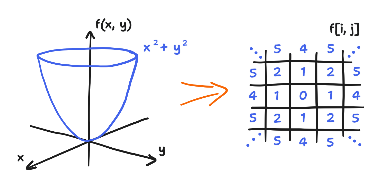
Side note: it’s a fair question to ask here why f[i, j] doesn’t correspond to—say—$(x_j, y_i)$ instead. Why does i select the horizontal component and not the vertical one? This is continuing from my discussion on the correspondence in my last post. The answer is that you could go about it that way and then derive a different but entirely consistent discretization. In fact, I originally had it that way. However, I switched out of that to keep all the expressions looking like how they do in the literature. So, in short, it’s convention.
Second side note: this is not to say that the array is a matrix. The array is only two-dimensional because the space is two-dimensional. If the space was three-dimensional, then so would be the array. And forget about arrays if the mesh isn’t a grid! So, most matrix operations wouldn’t mean anything either. It’d be more correct to think of discretized fields as very long vectors, but we’re encroaching on a next-post matter now.
Anyway, a key result of discretizing space is that the differential operators can be approximated by differences (i.e. subtraction) between the values of the field at a point and its neighbors. Furthermore, using a grid makes these differences incredibly simple by turning $\frac{\partial}{\partial x}$ into the value of the right neighbor minus the value of the left neighbor and $\frac{\partial}{\partial y}$ into the top minus the bottom. The methods that use this fact are “finite difference methods”, and the pressure step is one such method, but we’ll go into more detail on that in the next post.
So, to sum up this “just for context” moment, to compute an (approximate) solution to the presented partial differential equations, we need two levels of discretization. First, we need to discretize time, turning it into a scheme of updating the density and velocity fields repeatedly. Then, we need to discretize space to make the update computable. All this is because computers cannot handle functions of continuous time nor functions of continuous space, let alone functions of both like an evolving field. Now, all this is quite abstract, and that’s because each part invokes the discretization of time and space slightly differently, and we’ll go into the details of each.
With all that said, in the face of our definitions of $\frac{\partial \rho}{\partial t}$ and $\frac{\partial \bold v}{\partial t}$, this generally means that the density/concentration field (which I’m currently just calling the density field out of expediency) and the velocity field become just density and velocity arrays, and we must calculate their updates. In this situation, we update the arrays term by term, hence why each step of the overall process corresponds to a single term. (Though, I’m not sure if the implicit assumption of independence between the terms that underlies going term by term is just an expedient approximation or our math-given right. Anyway…) Let’s go over the four parts, step by step.
The first step is the “semi-Lagrangian advection” of the velocities, implementing the $-(\bold v \cdot \nabla) \bold v$ term. A key highlight here: Stam’s treatment of the advection term is not a finite differences method, yet it still uses discretization with a grid! I’d also like to highlight a bit of how Stam arrived at this method, though the GPU Gems chapter and Wong’s blog post would more succinctly jump to the end result. Now, I can’t do justice to the entire derivation. With that said, if you ever move on the reading Stam’s “Stable Fluids”, you’d find that Stam’s formal analysis involves a technique called a “method of characteristics”. It’s got a whole proof, but I’d just say that it looks like this: at every point $\bold x$ (that’s the coordinate vector $\bold x$, if you remember from Part 2), there is a particle that arrived there from somewhere. Letting $\bold{p}(\bold x, t)$ be its path—where the current location is given as $\bold{p}(\bold x, t_0) = \bold x$—then $\bold{p}(\bold x, t_0 - \Delta t)$ is where the particle was in the previous time.
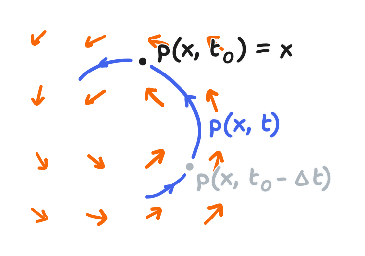
As a result, the particle must have carried its properties along the way, and one of them is said to be momentum, in other words, velocity. Therefore, an advection update looks like the assignment of the field value at $\bold{p}(\bold x, t_0 - \Delta t)$ to the field at $\bold x$. This result directly falls out of the assumptions that Stam presents (and for which I boorishly presented a picture instead), and it can be written as the following:
\[\bold{v}_\text{advect}(\bold x) = \bold{v}(\bold{p}(\bold x, t_0 - \Delta t))\]You may notice that Stam is presenting a unique time discretization here. You may also notice that it’s not computable yet because we’re missing a discretization of space. Of course, Stam presented one in “Stable Fluids” too. For starters, the calculation of $\bold{v}_\text{advect}$ can be done at just the points on the grid. From there, reading would show that Stam used a Runge-Kutta back-tracing on the velocity field to find $\bold{p}(\bold x, t_0 - \Delta t)$. I won’t get into how that works, and I won’t have to in a moment. Anyway, the found point almost certainly doesn’t coincide with a point on the grid, so Stam used an approximation of the velocity there, $\bold{v}(\bold{p}(\bold x, t_0 - \Delta t))$, by “bilinearly interpolating” between the four closest velocity values.
For more information on that, see the above link to Wikipedia. It’s got a better explanation of bilinear interpolation than one I can make—diagrams included. With that said, bilinear interpolation also amounts to very little code.
template<class T>
T billinear_interpolate(float di, float dj, T p11, T p12, T p21, T p22)
{
    T x1, x2, interpolated;
    x1 = p11*(1-dj)+p12*dj; // interp between lower-left and upper-left
    x2 = p21*(1-dj)+p22*dj; // interp between lower-right and upper-right
    interpolated = x1*(1-di)+x2*di; // interp between left and right
    return interpolated;
}
Though, a fair question to ask here: what should we do if the backtrace sends us to the boundary of the domain, or even beyond it? This is an important question because what we should do here directly depends on what the boundary is physically. In our case, the boundary is a solid wall. Here, I turn to the GPU Gems article, where it’s written that the “no-slip” condition hence applies, which just means the velocity there dmust be zero.
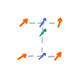
The no-slip condition can be implemented inside the bilinear interpolation scheme.
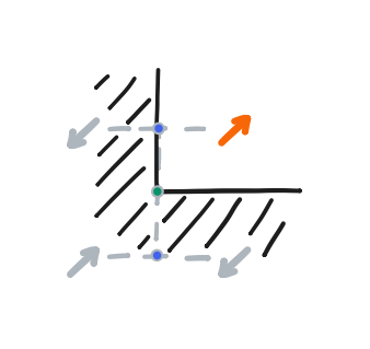
For now, let’s focus on the bottom row. Below the bottom row, we can construct a phantom row that always takes the negative of its values. Therefore, any linear interpolation at the halfway point between the bottom row and the phantom row must be equal to zero. That is, the halfway line between them achieves the no-slip condition, thereby simulating the solid wall. From there, if the backtrace gives a position that is beyond the halfway line, it should be clamped to it. This approach with the phantom row extends to all sides of the domain.
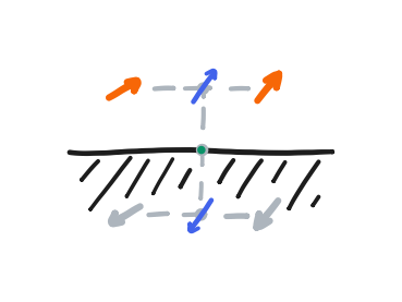
We also need to define the value of the phantom corner formed by a phantom row and phantom column. I didn’t see a rigorous treatment of them in my references, and I’ve seen that the corners might not matter much in practice. Still, the “no-slip” condition has a nice internal consistency that just gives us this definition. At the intersection of the halfway lines, the velocity there must also be zero. From this, we can form an equation involving the value of the phantom corner, and its solution is that the phantom corner should take on the value of the real corner—not its negative! Rather, it can be thought of as the phantom row taking the negative of the value at the end of the phantom column, which is itself a negative, and this makes a double negative.
This completes what Stam showed in “Stable Fluids”, though I pulled in the no-slip condition and its implementation from the GPU Gems article.
Regarding what we have so far: according to Stam, the “method of characteristics” update before discretization is “unconditionally stable” because no value in $\bold{v}_\text{advect}$ can be larger than the largest value in $\bold v$ (obviously because $\bold{v}_\text{advect}$ always is some value in $\bold v$), and his discretization with linear interpolation preserved the stability (because $\bold{v}_\text{advect}$ is always between some values in $\bold v$ or zero). This is especially important; in the past, I had written fluid simulations that didn’t have unconditional stability, and they blew up unless I took small timesteps. Getting to take large timesteps here is critical to running this sim on an ESP32.
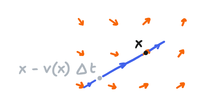
However, we’re one further approximation away from the method that appears in “Realtime Fluid Dynamics for Games” (and also the GPU Gems article and Wong’s post). Quite simply, if finding the path from $\bold{p}(\bold x, t_0 - \Delta t)$ to $\bold x$ can be called a nonlinear backtrace, then it’s replaced with a linear backtrace. The path is approximated with a straight line that extends from $\bold x$ in the direction of the velocity there:
\[\bold{v}_\text{advect}(x) = \bold{v}(\bold x - \bold{v}(\bold x) \Delta t, t)\]or in other words $\bold x - \bold{v}(\bold x) \Delta t$ replaces $\bold{p}(\bold x, t - \Delta t)$
This expression is shown as the principal discretization in the references I’ve mentioned—and it’s not hard to take it as so—but it’s really three parts: a “method of characteristics” analysis that comprises a time discretization, a space discretization using a grid and linear interpolation, and a further approximation using a linear backtrace. With these essential components in mind, we can draw a couple of conclusions:
- In “Realtime Fluid Dynamics for Games”, Stam goes on to state that “the idea of tracing back and interpolating” is a kind of “semi-Lagrangian method”, and so the linear backtrace isn’t quintessential to that classification. It remains a useful approximation, though.
- The key feature of this method is the unconditional stability that comes from the interpolation not exceeding the original values, and that’s a useful constraint to carry forward. For example, if you find yourself wasting compute on clipping values, like I once did, then something wasn’t done correctly.
- Generally speaking, this advection method isn’t the end-all and be-all of advection methods, and the field of fluid simulation is much larger than that. And it escapes me—go look to other sources for those.
In any case, this perspective doesn’t change the fact that the advection update fortunately manifests as only a couple of lines of C or C++. Here’s how I wrote it in ESP32-fluid-simulation.
template<class T, class VECTOR_T>
void semilagrangian_advect(Field<T> *new_property, const Field<T> *property, const Field<VECTOR_T> *velocity, float dt){
    int N_i = new_property->N_i, N_j = new_property->N_j;
    for(int i = 0; i < N_i; i++){
        for(int j = 0; j < N_j; j++){
            VECTOR_T displacement = dt*velocity->index(i, j);
            VECTOR_T source = {i-displacement.x, j-displacement.y};

            // Clamp the source location within the boundaries
            if(source.x < -0.5f) source.x = -0.5f;
            if(source.x > N_i-0.5f) source.x = N_i-0.5f;
            if(source.y < -0.5f) source.y = -0.5f;
            if(source.y > N_j-0.5f) source.y = N_j-0.5f;

            // Get the source value with billinear interpolation
            int i11 = FLOOR(source.x), j11 = FLOOR(source.y),
                i12 = i11, j12 = j11+1,
                i21 = i11+1, j21 = j11,
                i22 = i11+1, j22 = j11+1;
            float di = source.x-i11, dj = source.y-j11;
            T p11 = property->index(i11, j11), p12 = property->index(i12, j12),
                p21 = property->index(i21, j21), p22 = property->index(i22, j22);
            T interpolated = billinear_interpolate(di, dj, p11, p12, p21, p22);
            new_property->index(i, j) = interpolated;
        }
    }
    new_property->update_boundary();
}
We can see the linear backtrace in the calculation of the source vector. The source vector is floating-point, but the arrays are indexed with integers. So, I used the FLOOR macro to find the upper-left point, and then I found the rest by adding one. I wrote FLOOR to calculate the floor function, and—no—it’s not the same as (int)x! (int)x rounds toward zero, and the floor function strictly rounds down. Finally, there’s also clamping of the source vector and new_property->update_boundary() which calculates the phantom rows and columns.
It’s worth noting that, because semi-Lagrangian advection is also applied to the density later, that step can be implemented using the same code that does velocity advection. If you look at the terms $-(\bold v \cdot \nabla) \bold v$ and $-(\bold v \cdot \nabla) \rho$, you can see that the operator doesn’t change—only what’s being operated on does. The only difference is that the “no-slip” condition doesn’t apply to advecting density, so the phantom rows and columns should just copy instead of taking the negative.
Personally, I took the natural approach for C++ and wrote a function template, and that meant it could take either the density array or the velocity array. Then, I had the new_property->update_boundary() method either do the copy or the negative, depending on a private variable of new_property. You can see how that works in the Field.h file of ESP32-oled-spectrum. That said, an approach that also works in C is to recognize $x$-velocity and $y$-velocity as independent properties. Then, they can be stored in separate, scalar arrays—say u and v—and then the same code that operates on density arrays can operate on each component. You can see how exactly that would it would be done in “Realtime Fluid Dynamics for Games”.
Moving on from the semi-Lagrangian advection of velocity (and density), the second step is to apply the user’s input to the velocity array. This corresponds to the $\bold f$ term, the external forces term. This isn’t something Stam had set in stone, since what makes up the external forces really depends on the physical situation being simulated. In our case, we want someone swirling their arm in the water, and so external forces must be derived from the touch data. That’s the touch data we had the touch task generate in Part 2, and here’s where it comes into play.
Recall that a touch input consists of a position and a velocity. Let $\bold{x}_i$ and $\bold{v}_i$ be the position and velocity of the $i$-th input in the queue. Naturally, we should want to influence the velocities around $\bold{x}_i$ in the direction of $\bold{v}_i$. Under this general guidance, I could have gone about it in the way that was done in the GPU Gems article. That was to add a “Gaussian splat” to the velocity array, and that “splat” was formally expressed as something like this
\[\bold{f}_i \, \Delta t \, e^{\left\Vert \bold{x} - \bold{x}_i \right\Vert^2 / r^2}\]where $\bold{f}_i$ is a vector with some reasonably predetermined magnitude but a direction equal to that of $\bold{v}_i$. From the multiplication $\bold{f}_i \Delta t$, you may notice that the time discretization in play is just Euler’s method and that the space discretization in play is to just evaluate it at the points of the grid. Across all the inputs in the queue, the update would have been
\[\bold{v}_\text{force}(\bold{x}) = \bold{v}(\bold{x}) + \sum_{i = 0}^n \bold{f}_i \, \Delta t \, e^{\left\Vert \bold{x} - \bold{x}_i \right\Vert^2 / r^2}\]where $n$ is the number of items in the queue. I had two issues with it. First, I specifically wanted to capture how you can’t push the fluid faster than the speed of your arm in the water. This was especially important when someone was moving the stylus very gently. Second, evaluating the splat at every single point would’ve been expensive. My crude solution to this was to just set $\bold{v}(\bold{x}_i)$ to be equal to $\bold{v}_i$. In code, that turns out to merely be the following
struct touch current_touch;
while(xQueueReceive(touch_queue, ¤t_touch, 0) == pdTRUE){ // empty the queue
velocity_field->index(current_touch.coords.y, current_touch.coords.x) = {
.x = current_touch.velocity.y, .y = current_touch.velocity.x};
}
velocity_field->update_boundary(); // in case the dragging went near the boundary, we need to update it
where, if you’re confused about the apparent “axes swap”, see the section in Part 2 about the AdafruitGFX coordinate system. Formally, I can write this code as as
\[\bold{v}_\text{force}(\bold{x}_i) = \bold{v}_i\] \[\bold{v}_\text{force}(\bold{x}) = \bold{v}(\bold{x}) \text{ for } \bold{x} \not= \bold{x}_i \text{ for any } i\]The third step is the pressure step, corresponding to the $- \frac{1}{\rho} \nabla p$ term. Out of all the terms in the definition of $\frac{\partial \bold v}{\partial t}$, it must be calculated last, capping off the velocity update before we can proceed to the density update. I already discussed this in Part 2, but in short, the pressure does not represent a real process here. Rather, it is a correction term that eliminates divergence in the velocity field. This ensures the incompressibility constraint, $\nabla \cdot \bold v = 0$. (Technically, the specific formulation that Stam presents doesn’t eliminate it entirely, but it does eliminate most of it. We can get into that in the next part.) Since it’s not a real process, no time discretization is in play. Rather, the updated velocity field is straight-up not valid until the correction is applied.
It would be more correct to state that Stam’s fluid simulation follows the modified definition that he presents in “Stable Fluids”, that is
\[\frac{\partial \bold v}{\partial t} = \mathbb{P} \big( - (\bold v \cdot \nabla) \bold v + \nu \nabla^2 \bold v + \bold f \big)\]where $\mathbb{P}$ is a linear projection onto the space of velocity fields with zero divergence. This definition clearly shows that $\mathbb{P}$ must be calculated last, though it hides the fact that calculating it does involve a gradient. Anyway, applying the reductions that we’ve been running with so far, that would just be
\[\frac{\partial \bold v}{\partial t} = \mathbb{P} \big( - (\bold v \cdot \nabla) \bold v + \bold f \big)\]where, we’ve again set $\nu$ to zero.
This happens the pressure projection is shown in the GPU Gems chapter. That said, to keep the notation simple, I won’t continue to use it. And on the matter of actually calculating it, there’s so much to say in the next part. I’ll provide the code then as well.
That just leaves the fourth and final step, the semi-Lagrangian advection of the density, corresponding to the term $-(\bold v \cdot \nabla) \rho$. Well, we’ve made it the only term in the definition of $\frac{\partial \rho}{\partial t}$, and we’ve already implemented it. There are no more obstacles here. The only thing I’d mention is that extending the fluid sim to full color is quite trivial. Instead of advecting a single density field, we can advect three density fields—one for red dye, one for blue dye, and one for green dye.
That fills most of the outline, implementing every part of the reduced Navier-Stokes equations except for the pressure step. That’s the applied force and the semi-Lagrangian advection of the velocity and density. There, we paid special attention to the derivation and the no-slip boundary condition, since that comes from the physical situation being simulated. We also went a bit into the general idea of discretizing time (i.e. numerical integration) and discretizing space in order to give context. That’s everything I know about those steps that I think could help their implementation. In the next and final post, we’ll go over what, exactly, the pressure step is, including the relevant linear algebra. Stay tuned!