Rebuilding ESP32-fluid-simulation: the touch and render tasks (Part 2)

So, how exactly did my rebuild of ESP32-fluid-simulation do the touch and render tasks? This post is the second in a series of posts about it, and the first was a task-level overview of the whole project. But while it’s nice and all to know the general parts of the project and how they communicate in a high-level sense, the meat of it is the implementation, and I’m here to serve it. The next parts are dedicated to the sim physics, but we’ll talk here about the input and output: the touch and screen of a touchscreen.

The implementation starts from the hardware, naturally. As I established, I went with the ESP32-2432S032 development board that I heard about on Brian Lough’s Discord channel, where it was dubbed the “Cheap Yellow Display” (CYD). That choice guided the libraries that I was going to build on, and that defined the coding problems I had to solve.

The ESP32-2432S032, a.k.a. the Cheap Yellow Display

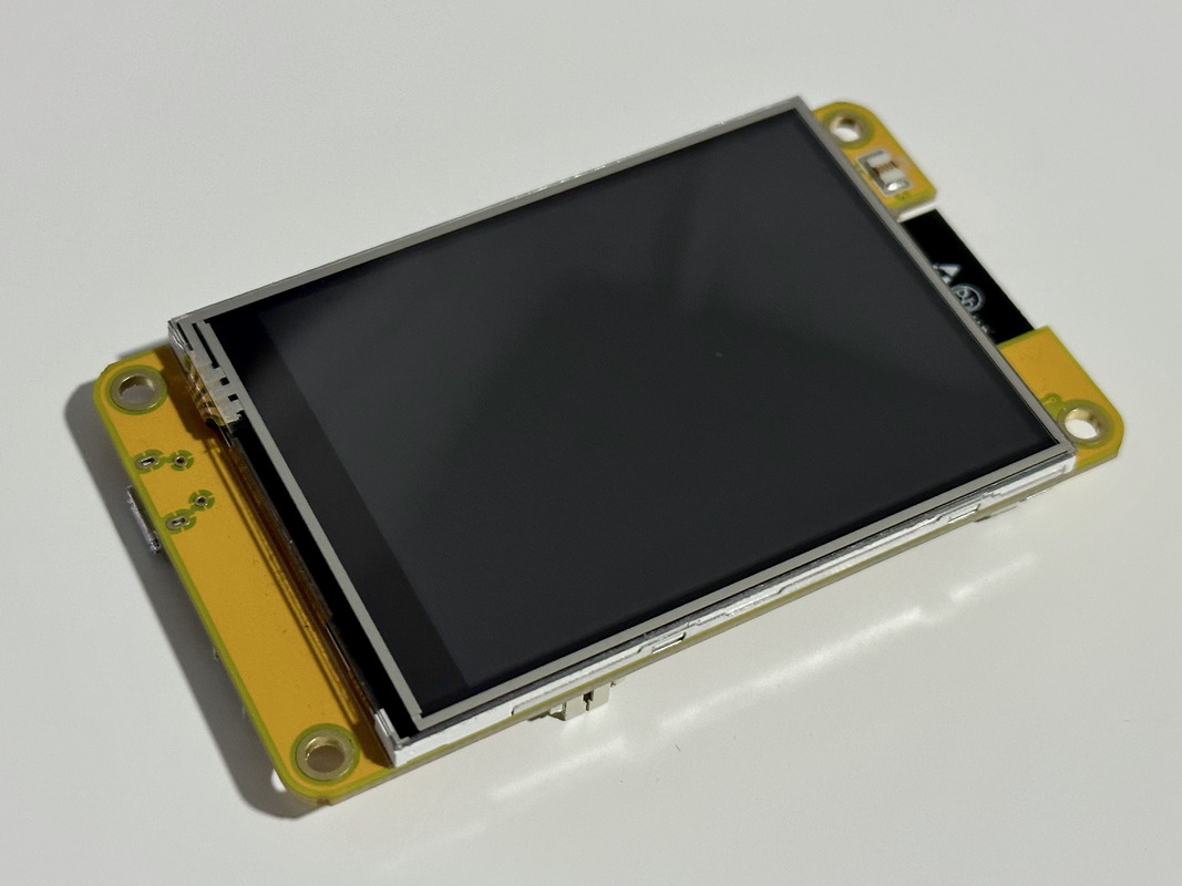
Materially, the only component of it that I used was the touchscreen, and it used an ILI9341 LCD driver and an XPT2046 resistive touchscreen controller. In some demonstrative examples, Lough used the TFT_eSPI library to interact with the former chip and the XPT2046_Touchscreen library for the latter chip, and these examples included what pins and configuration to associate with each. None of this setup I messed with.

We can cover the touch task first. To begin with, I already had a general idea for what it should do: a user had to be able to drag their stylus across the screen and then see water stirring as if they had stuck their arm into it and whirled it around in reality. With that in mind, what should we want to capture, exactly?

The objective can be split into three parts. First, we should obviously check if the user is touching the screen in the first place! Second, assuming that the user is touching the screen, we should obviously get where they touched the screen. Finally, if we keep track of the previous touch location, we can use it later to estimate how fast they were dragging the stylus across the screen—assuming they were, that is. We’ll get to that in a bit.

To deal with the first two matters, reading the documentation for the XPT2046_Touchscreen library takes us most of the way. A call to the .touched() method tells us whether the user touched the screen. Assuming this returns true, getting the where is just a call to the .getPoint() method. It returns an object that contains the coordinates of the touch—coordinates that we’ll need to further process.

First, we should quickly note that the XPT2046 always assumes that the screen is 4096x4096, regardless of what the dimensions actually are. That can just be fixed by rescaling. To be exact, the getPoint() method returns a TSPoint struct with members .x, .y, and .z. Ignoring .z, we first multiply .x by the screen width and .y by the height. (In fact, I multiplied them by a fourth of that because I had to run the sim at sixteenth-resolution, but that’s beside the point.) Then, we divide .x and .y by 4096. Rescaling in this way, multiplying before dividing, preserves the most precision.

With that said, you’re free to ask here: why should .x be multiplied by the width, and .y by the height? That would imply that .x is a horizontal component and .y is a vertical component, right? That’s correct, but a surprising complication comes from the fact that we’re feeding a fluid sim.

The second thing we need to do is recognize that the XPT2046_Touchscreen library is written to yield coordinates in the coordinate system established by the Adafruit_GFX library. It’s a somewhat niche convention that has tripped me up multiple times despite how simple it is, so I’ll cover it here.

The Adafruit_GFX library has set conventions that are now widespread across the Arduino ecosystem. Even up to function signatures (name, input types, output types, etc), the way to interact with adhering display libraries doesn’t change from library to library—save a couple of lines or so. For example, my transition of this project from an RGB LED matrix to the CYD was trivial, yet there couldn’t be more of a gap between their technologies. This is because the libraries I used for them, Adafruit_Protomatter and TFT_eSPI respectively, adhered to the conventions.

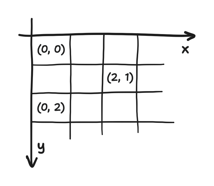
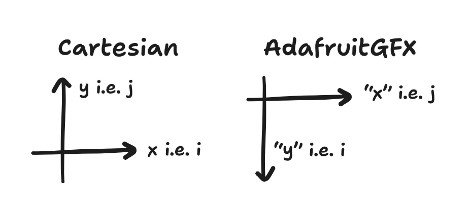
One of these conventions is their coordinate system. When I say coordinate system, “Cartesian” might be the word that pops into your mind, but the Cartesian coordinate system was not what Adafruit_GFX used, even though they do refer to pixels by “(x, y)” coordinates. In the ordinary Cartesian system, the positive-x direction is rightwards, and the positive-y direction is upwards. They had them be rightwards and downwards respectively.

This should be compared to the way a 2D array is indexed in C. Given the array float A[N][M], A[i][j] refers to the element i rows down and j columns to the right. This notation is just a fact of C, but to keep things clear in a moment, I’ll refer to it as “matrix indexing”.

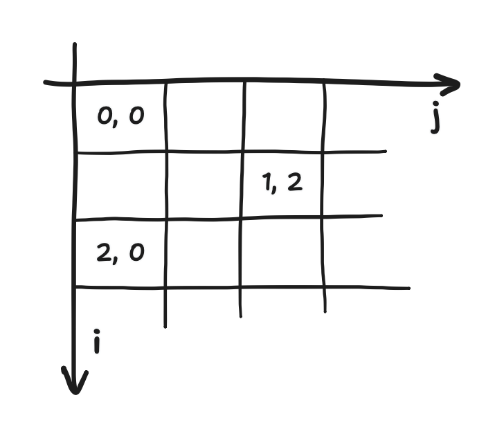
Note: i and j are represented in this diagram as "i, j"

In a way, we can think of i and j as coordinates. In fact, if we equate i to “y” (the downward-pointing one used by Adafruit_GFX, which I’m writing here in quotes) and j to “x”, then I’d argue that matrix indexing and the Adafruit_GFX coordinates are wholly equivalent—as long as we adhere to this rename. Well, we don’t end up sticking with it, actually.

We’ll cover this in more depth in the next posts, but it turns out that the type of fluid simulation I’m using is constructed on a Cartesian grid which doesn’t use matrix indexing. Points on the grid are referred to by their Cartesian coordinates (x, y), exactly as you’d expect. It’s also starkly different from the Adafruit_GFX coordinates “(x, y)”. (In this article, I’ll write (x, y) when I mean the Cartesian coordinates and “(x, y)” when I mean the Adafruit_GFX coordinates.) At the same time, i and j can be used to refer to the point on the grid at the i-th column from the left and the j-th row from the bottom. I’ll refer to it as “Cartesian indexing”.

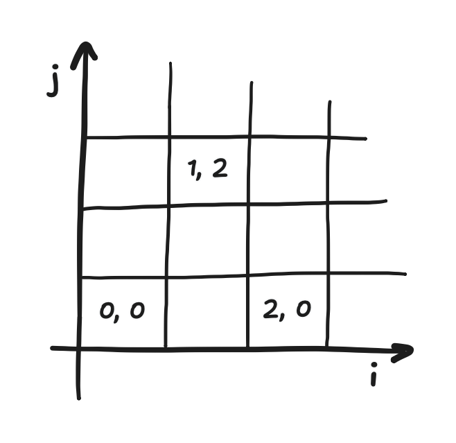
Note: i and j are represented in this diagram as "i, j"

Increasing i moves you rightward, and increasing j moves you upward. In other words, i specifies the x-coordinate, and j specifies the y-coordinate. This correspondence between Cartesian coordinates and Cartesian indexing is flipped, roughly, from the correspondence between Adafruit_GFX coordinates and matrix indexing. It’s not an exact reversal because that postitive-y means up while positive-“y” means down.

The axes of matrix and Cartesian indexing

What does this mean for us? What’s the consequence? We need to change coordinate systems i.e. transform the touch inputs. Fortunately, I’ve found a cheap trick for this. If you look at the i’s and j’s in the above diagram (and set aside the conflicting x’s and y’s), you may suspect that the transform we need to do with a rotation. I did try this, and it did work. That said, the trick is to know that the physics doesn’t change if we run the simulation on a space that is itself rotated.

With the trick, the screen and sim no longer operate on the same space, but corresponding points have the same coordinates/indices. Without the trick, points in the shared space have different coordinates/indices for the sim and screen.

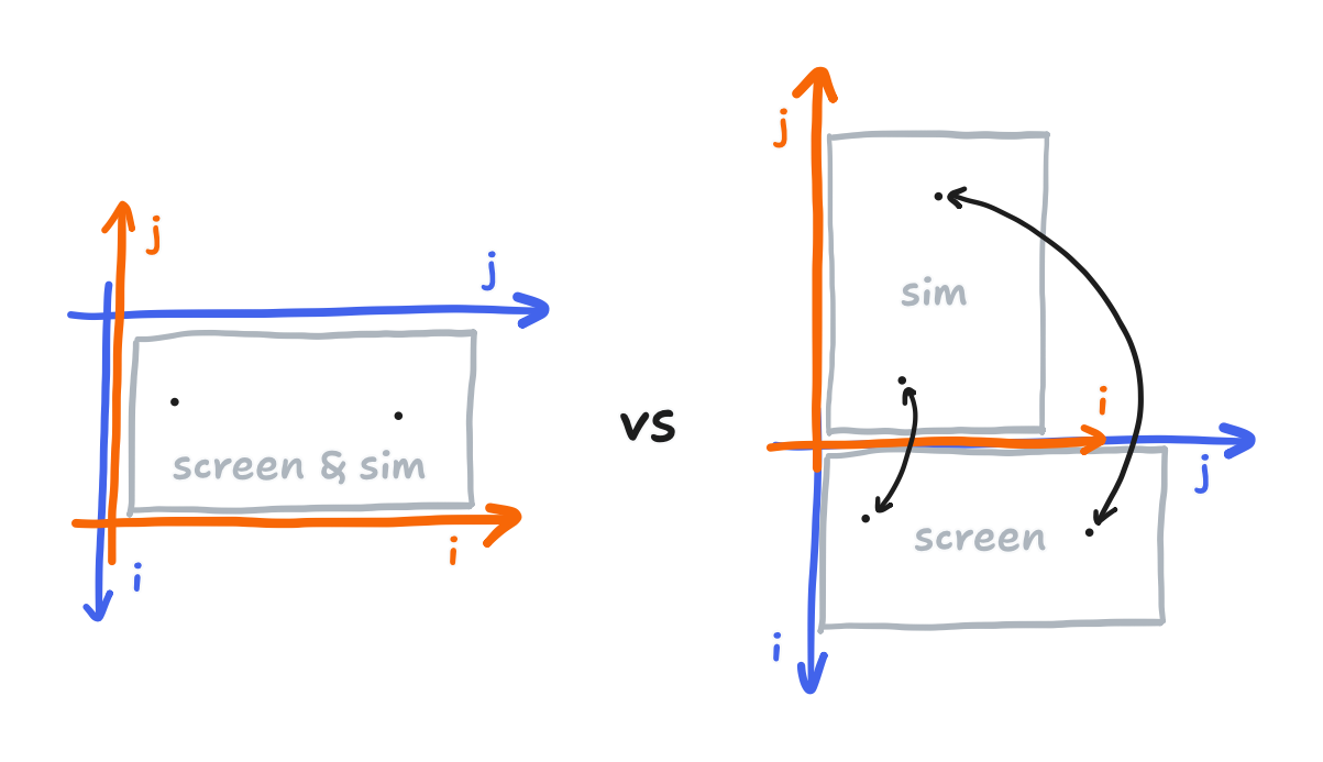
Going about it this way, the i and j of a pixel on the screen, using matrix indexing, and the i and j of a point in the simulation space, using Cartesian indexing but also being rotated relative to the screen, are identical. With this trick, the transform is to do nothing! (If we speak in x, “x”, y, and “y”, instead, then that’s a swap of the axes, but it’s more like swapping labels.)

It also happens here that the actual arrays used for sim operations are now the same shape as the arrays used for screen operations. This comes from the correspondences we mentioned before being flipped.

Combining the physical rotation of the sim space with the scaling that also accounts sim being sixteenth-resolution, we now have taken a touch from the XPT2046 format to the sim space.

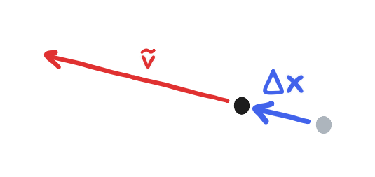
That leaves the third part to capture: an estimate of the velocity. There is nothing built in for this, so I had to tease out one out. An idea that I exploited to get it is that, as the stylus is dragged across the screen, it had to have traveled from where we last observed a touch to where we see a touch now. This is a displacement that we divide by the time elapsed to get an approximation of the velocity. To use vector notation, we can write this as the expression

\[\tilde {\bold v} = \frac{\Delta \bold x}{\Delta t}\]

where $\Delta t$ is the time elapsed and $\Delta \bold x$ is a vector composed of the change in the $x$-coordinate and the change in the $y$-coordinate. (We can use either coordinate system’s definition of x and y for this, trick or not.) This approximation gets less accurate as $\Delta t$ increases, but I settled for 20 ms without too much thought. I just enforced this period with a delay.

Appoximating the current velocity with the previous displacement

That said, the caveat is that this idea doesn’t define what to do when the user starts to drag the stylus, where there is no previous touch. Strictly speaking, we can save ourselves from going into undefined territory if we code in this logic: if the user was touching the screen before and is still touching the screen now, then we can calculate a velocity, and in all other cases (not now but yes before, not now and not before, and yes now but not before) we cannot.

Finally, if we had detected a touch and calculated a velocity, then the touch task succeeded in generating a valid input, and this can be put in the queue to be served to the sim!

That leaves the render task, using the TFT_eSPI library. We’ll again cover this in a future part, but the fluid simulation puts out individual arrays for red, green, and blue, but they together represent the color. Let’s say that I had full-resolution arrays instead of sixteenth-resolution ones. Then, we’ve already set the sim up such that we need not do anything to change coordinate systems. Every pixel on the screen is some i rows down and some j columns to the right, and its RGB values can be found at (i, j) in the respective arrays. The approach would be to go pixel by pixel, indexing into the arrays with the pixel’s singular i and j, encoding the RGB values into 16-bit color, and then sending it out. It would have been as simple as that.

Now, let’s reintroduce the fact that we only have sixteenth-resolution arrays.

Because this now means that the arrays correspond to a screen smaller than the one we have, we have a classic upscaling problem. There are sophisticated ways to go about it, but I went with the cheapest one: each element in the array gets to be a 4x4 square on the screen. From what I could tell, it was all I could afford. Because it meant that the 4x4 square was of a single color, I could reuse the encoding work sixteen times! Really though, if I had more computing power, I suspect that this would’ve been an excellent situation for those sophisticated methods to tackle.

This choice of upscaling alone might offer a fast enough render of the fluid colors, especially if we batch the 16 pixels that make up the square into a single call of fillRect(). That’s one of the functions that was established by Adafruit_GFX. However, I found that I needed an even faster render, so I turned to some features that were unique to TFT_eSPI: “Sprites” and the “direct memory access” (DMA) mode.

Now, googling for “direct memory access” is bound to yield what it is and exactly how to implement it, but to use the DMA mode offered by TFT_eSPI, we only need to know the general idea. That is, a peripheral like the display bus can be configured to read a range of memory without the CPU handling it. For us, this means we would be able to construct the next batch of pixels while the last one is being transferred out. However, to do this effectively, we’ll need to batch together more than just 16 pixels.

That’s where “Sprites” come in. Yes, you might think of pixel-art animation when I say “sprites”, but here, it’s a convenient wrapper around some memory. Presenting itself as a tiny virtual screen, called the “canvas”, it offers the same functions that we can expect from a library following Adafruit_GFX. As long as we remember to use coordinates that place the square in this canvas (and not the whole screen!), we can load it up with many squares using the same fillRect() call, but under the hood, no transferring takes place yet. Once this sprite is packed with squares, only then do we initiate a transaction with a single call to pushImageDMA(), this function invoking the DMA mode. From there, we can start packing a new batch of squares at the same time.

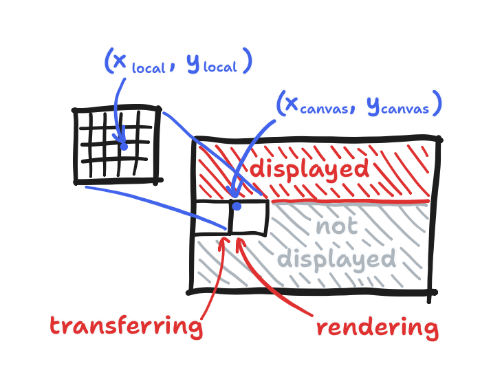
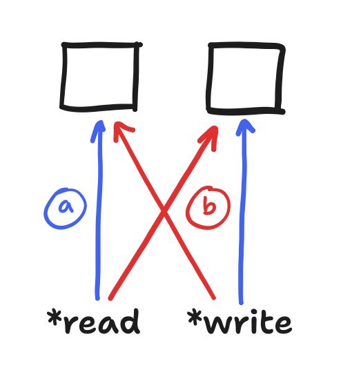
fillRect() is called with (x_local, y_local) as where the square starts, pushImageDMA is called later with (x_canvas, y_canvas) as where the sprite starts, and meanwhile the previous sprite is still transferring

The caveat: if we pack squares into the same memory that we’re transferring out with DMA, then we’d end up overwriting squares before they ever reach the display. Therefore, we’d want two sprites—one for reading and one for writing—and then we’d flip which gets read from and which gets written to. This flip would happen after initiating the transaction but before we start packing new squares. Finally, the terminology for this is “double buffering”, more specifically that’s the “page flipping” approach to it, but the purpose of it here is more than just preventing screen tearing.

Classical page flipping is two buffers and two pointers: no data is copied between the buffers but the pointers get swapped.

That covers the touch and render tasks, altogether describing how I used the touchscreen module. But between the hardware and my code are the TFT_eSPI and XPT2046_Touchscreen libraries, and that set in stone the features and conventions I got to work with. In particular, I had to lay out the exact relationship between Cartesian indices and the “(x, y)” Adafruit_GFX coordinates that have become ubiquitous across Arduino libraries, in large part because of the Adafruit_GFX library. With the rotation trick, we eliminated the transform between them. With that in mind, using XPT2046_Touchscreen was just a matter of scaling and maintaining a bit of memory. On the other hand, I turned to the DMA mode and “Sprites” that were uniquely offered by the TFT_eSPI library just to keep pace. Those features also kept within the Adafruit_GFX box, so just a bit of extra care (double buffering, that is) was needed.

With this post and the last post done, there’s one last task to cover: the next post is an overview of the physics before we get into the implementation. Stay tuned! But if you’re here before that post comes out, there’s always the code itself on Github.