Recoloring backgrounds to align with the Solarized base palette again (plus color, light mode support, and a demo!)
A couple of months back, I wrote “Recoloring backgrounds to align with the Solarized Dark base palette”, and when I wrote that I wasn’t expecting to do a second part. At the time, because I had just encountered the Solarized palette, I didn’t even begin to fathom how you could add colors to the backgrounds. Still, even then I could imagine what it would look like, and shortly after I wrote that article I started to go down what seemed like the right path. I found myself making a 3D scatter plot of the entire Solarized palette as CIELAB values, and it looked to me like a spinning top in the middle of falling over.
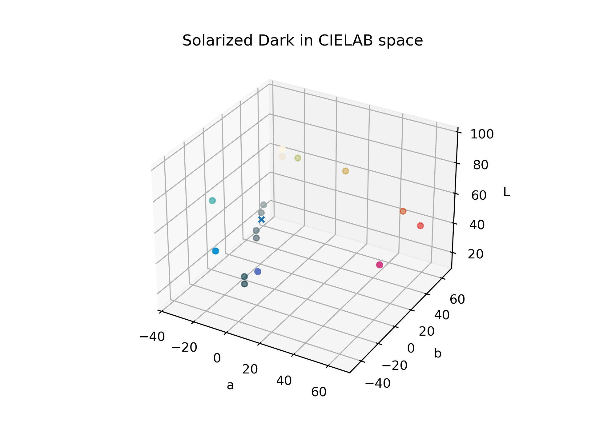
So, I thought that all I might need to do was transform the colors of an image into points in CIELAB space, tip them over just the same, and then transform them back into RGB color. However, I didn’t come around to trying that idea until now. After a great deal of experimentation, I’ve found a particular style of “solarizing” images that generally works for any image: start by following the monochrome scheme that aligns with the Solarized base palette, then allow some subtle tinting with the other colors.
You can try it for yourself using a demo I put on HuggingFace.
Ultimately, it didn’t just involve tipping over a top. The general outline for achieving the effect is this:
- Transform the colors of the image into points in CIELAB space,
- reduce their saturation/”chroma” component,
- remap their lightness component,
- rotate and shift them (still in CIELAB space), and finally
- transform them back into RGB color.
It’s worth noticing here that all the work was done in CIELAB space. It is the coordinate space in which the Solarized palette was canonically defined, but it’s also a space with a very convenient property. That is: the lightness of a color is an independent component. Out of the components of a point in CIELAB space, $L$, $a$, and $b$, lightness is just $L$. Given some—say—purple, you can get the same purple but brighter or darker by varying just $L$, and you leave the $a$ and $b$ components alone. If we worked in RGB instead, we would have to vary the red, green, and blue components together.
The $a$ and $b$ components together form a plane of all possible mixtures of the primary colors, and a specific $a$ and $b$ mean a specific mixture. Going in the $+a$ direction gets a redder mixture. The $-a$ direction gets a greener mixture. $+b$ gets a yellower one, and $-b$ a bluer one. That said, in this case, we should think about the $a-b$ plane in polar coordinates. In polar, the angle is called the “hue” (the very same hue that you’d pick from a color wheel), and the magnitude is called the saturation or “chroma”.
The $L$, $a$, and $b$ components all have meanings that make each step of the process into simple operations. On top of that, scikit-image gives us convenient functions that step in and out of CIELAB space, called rgb2lab and lab2rgb respectively. That’s the advantage of working in CIELAB space. With that in mind, what are we trying to do in each step? We’ll want to cover this backward, starting with the shift and rotate—the meat of the method!
In my previous post, I chose to throw out color, and then I mapped the grayscale values onto the line going through the Solarized base palette in CIELAB space.
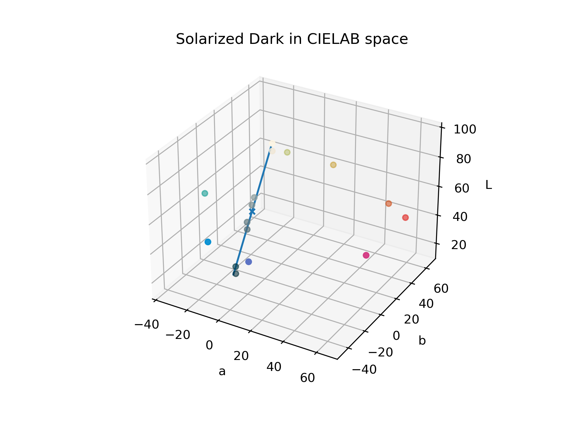
However, all grayscale values can be thought of as the line where $a=0$ and $b=0$, or in other words the $L$-axis, and “throwing out color” can simply be thought of as a linear projection of all values onto it. Because we can think of the Solarized base palette as a line and all grayscale values as another line, a similar (but not the same) way to do what I did before is to do the projection then apply an “affine” function. “Affine” functions take the general form
\[y = Ax+b\]and they differ from linear functions (their general form being $y=Ax$) only by a translation, expressed as the additional term $b$. Using an affine function makes sense here because the canonical center of CIELAB space is $(50, 0, 0)$, not the origin. (For that matter, the center of the Solarized base palette isn’t the origin either.)
On the mention of an affine function, you might follow up that thought by solving for A and b, perhaps by using a linear algebra package. In fact, though we have the Solarized base palette to possibly serve as $y$, we have nothing to serve for $x$. Before anyone mentions it, the Solarized website shows the colors it replaces for the xterm program, but a different set of colors of a different program can be replaced by the Solarized palette just the same. If we took the xterm colors as $x$, then we can just as arbitrarily take the colors of Google Chrome or Visual Studio Code as $x$. That is to say again: we have no solid choice for $x$. In that way, we’re forced to give up on using data to determine $A$ and $b$.
Instead, let’s give $A$ and $b$ some value, but we’ll guide our choice with some intuition. We’ll start with this: since we already know the center of CIELAB space and the center of the Solarized base palette, we can rewrite the affine transform as
\[y - y_0 = A (x - x_0)\]where we should notice that we implicitly set $b$ to $y_0 - A x_0$. This intuitively defines $b$ as whatever brings the center of $Ax$ from $A x_0$ to $y_0$.
That leaves defining $A$. Given that we’re passing in $x-x_0$ and getting out $y-y_0$, subtraction of the centers $x_0$ and $y_0$ means we’re actually passing in a line through the origin and getting out a different line through the origin. The natural operation that should come to mind here is rotation.
One definition of a rotation matrix is parameterized by yaw, pitch, and roll
\[\begin{align*} A & = \underbrace{ \begin{bmatrix} \cos\alpha & -\sin\alpha & 0 \\ \sin\alpha & \cos\alpha & 0 \\ 0 & 0 & 1 \end{bmatrix} }_\text{yaw} \underbrace{ \begin{bmatrix} \cos\beta & 0 & \sin\beta \\ 0 & 1 & 0 \\ -\sin\beta & 0 & \cos\beta \end{bmatrix} }_\text{pitch} \underbrace{ \begin{bmatrix} 1 & 0 & 0 \\ 0 & \cos\gamma & -\sin\gamma \\ 0 & \sin\gamma & \cos\gamma \end{bmatrix} }_\text{roll} \\ & = \begin{bmatrix} \cos\alpha \cos\beta & \cos\alpha \sin\beta \sin\gamma - \sin\alpha \cos\gamma & \cos\alpha \sin\beta \cos\gamma - \sin\alpha \sin\gamma \\ \sin\alpha \cos\beta & \sin\alpha \sin\beta \sin\gamma + \cos\alpha \cos\gamma & \sin\alpha \sin\beta \cos\gamma - \cos\alpha \sin\gamma \\ -\sin\beta & \cos\beta \sin\gamma & \cos\beta \cos\gamma \end{bmatrix} \end{align*}\]where $\alpha$, $\beta$, and $\gamma$ are the yaw, pitch, and roll angles respectively.
In my previous post, I found that the principal component of the Solarized base palette line was $(0.9510, 0.1456, 0.2726)$. For the $L$-axis, we can just take $(1, 0, 0)$ as the unit vector that spans it. Since these two vectors are unit-length, we can say that the rotation matrix is such that
\[\begin{bmatrix} 0.9510 \\ 0.1456 \\ 0.2726 \end{bmatrix} = A \begin{bmatrix} 1 \\ 0 \\ 0 \end{bmatrix}\]Solving for $\alpha$, $\beta$, and $\gamma$ yields
\[\begin{bmatrix} 0.9510 \\ 0.1456 \\ 0.2726 \end{bmatrix} = \begin{bmatrix} \cos\alpha \cos\beta \\ \sin\alpha \cos\beta \\ -\sin\beta \end{bmatrix}\] \[\begin{align*} \alpha & = 0.152 \\ \beta & = -0.275 \\ \gamma & \text{ is free} \end{align*}\]where we happen to find that roll about the $L$-axis, or in other words hue rotation, doesn’t matter! Let’s just let $\gamma = 0$.
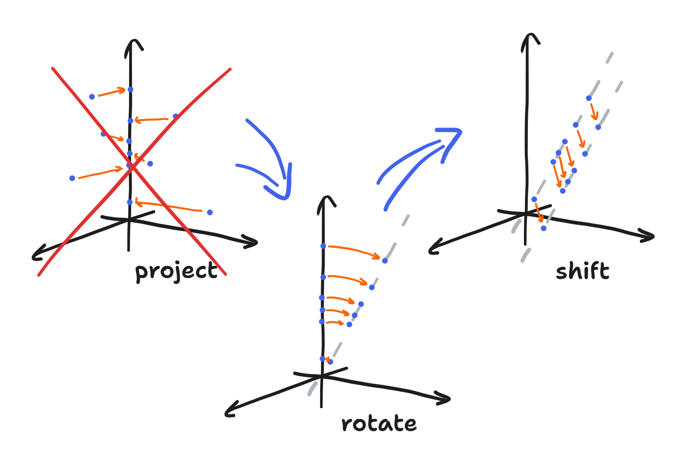
We’ve now fully defined the shift and rotate, that being an affine transform. Therefore, we could now get something like my old post while working entirely in CIELAB space. Instead, remember that we could throw out colors by projecting onto the $L$-axis? To get colors, we just don’t do that and then proceed with the shift and rotate anyway! Let’s visualize what we’ve done so far with the help of this diagram.
Now, what about the preprocessing steps?
Let’s look at the lightness remap first. Solarized is a low-contrast palette that offers a light mode and a dark mode. If we flip to the development section of the Solarized documentation, we find that it does so by assigning an upper and lower subset (not mutually exclusive) of the base palette to each respectively.
Given one mode or another, a fair expectation is that colors exclusive to the alternate mode are never encountered or else the theme is not low-contrast! For the same reason, we shouldn’t expect colors that are outside both palettes as well. Therefore, we need to restrict the range in which we expect points going through the rotate and shift to land, and that target range is a segment of the line going through the base palette along with the neighborhood around that segment.
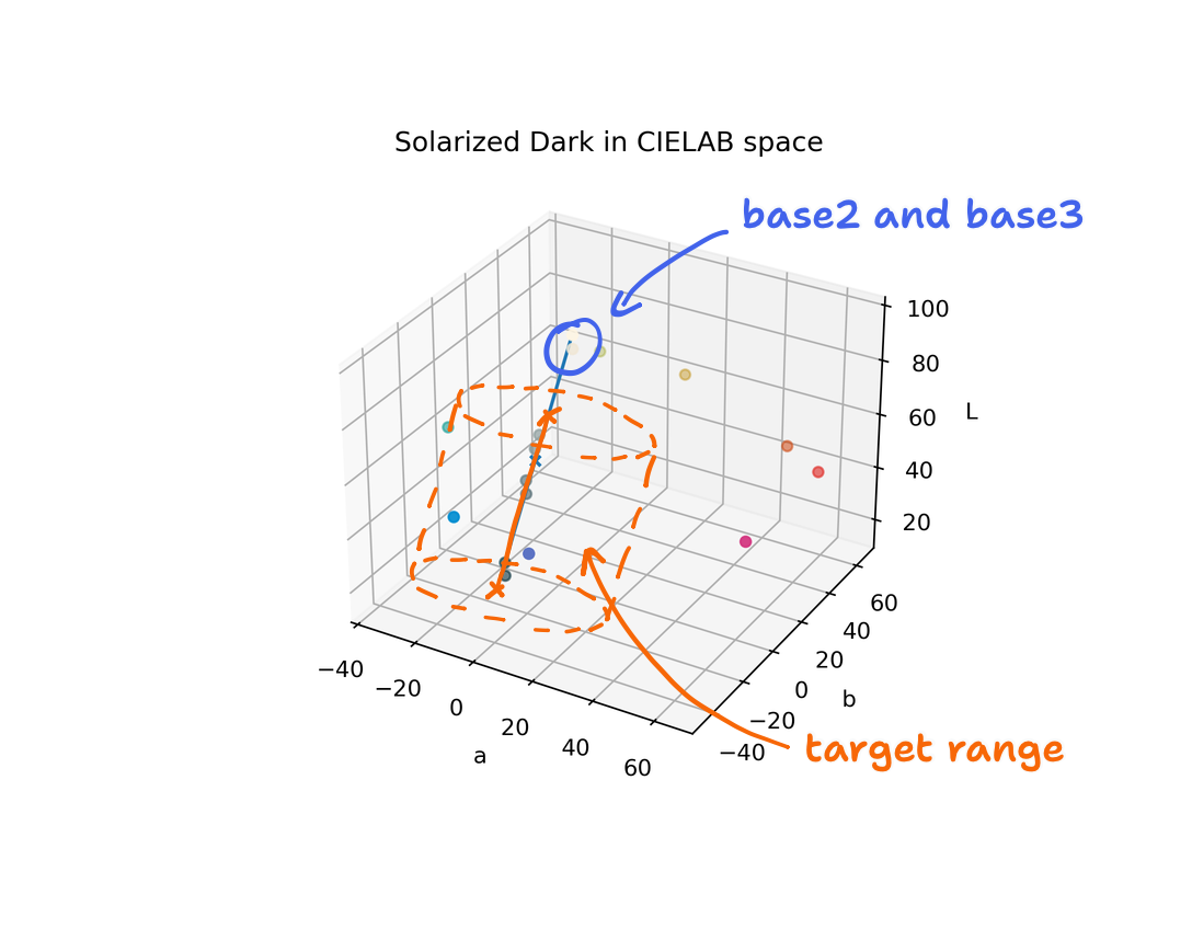
Taking the dark mode first, the target range is the segment between base03 and base1—excluding the brightest base2 and base3—and the neighborhood around it. We can invert the rotate and shift to find what values on the $L$-axis they correspond to. That’s how we find that the condition for achieving the target range is $8.1397 < L < 59.4372$. Therefore, if we remap the points of the input such that their lightness components fall into that range, we’re golden. The remap is
where $100$ and $0$ are the maximum and minimum possible lightness. On top of that, we don’t need to touch the $a$ and $b$ components. However, this remap may as well be the definition of destroying contrast, and breaking out of the target range a bit may be worth it. Taking $8.1397 < L < 59.4372$ as just a guideline, we can bounce between setting a new remap and generating a histogram until the distribution of lightnesses mostly falls in that range. I’ve provided an interface for that tweaking on HuggingFace, and we can go through an example in a moment.
Taking the light mode, the target range is between base01 and base3, ignoring base03 and base02, and this corresponds to a target lightness of $38.7621 < L < 93.8699$. The rest of the process is the same.
Finally, what about reducing the chroma? We do that to enforce the style, and that called for subtle tinting. As I mentioned before, when we rewrite the $a$-$b$ coordinates as polar coordinates, the chroma is the magnitude and the hue is the angle. So, cutting the chroma by some factor means cutting the magnitude of the $a$-$b$ coordinate. Of course, cutting the $a$ component and the $b$ component each by the same factor is equivalent. If we let the factor by which we cut the chroma be $\mu$, then
\[a_\text{new} = \mu a \qquad b_\text{new} = \mu b\]where I’ve found that $\mu = 0.25$ is a factor I like.
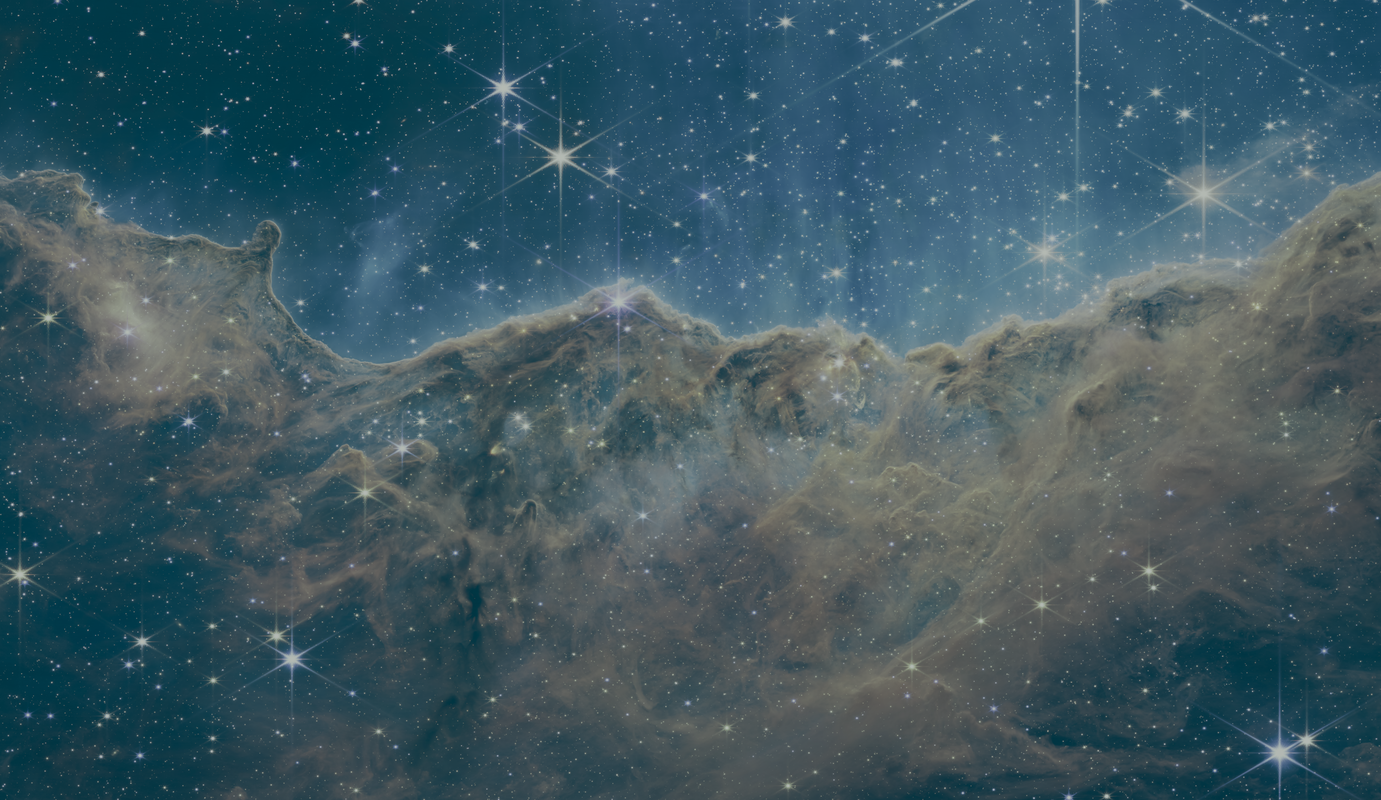
So, that’s the entire process for “solarizing” a background image defined. Let’s step through it in order with an example to review. We can input the Carina Cliffs into the Huggingface demo.
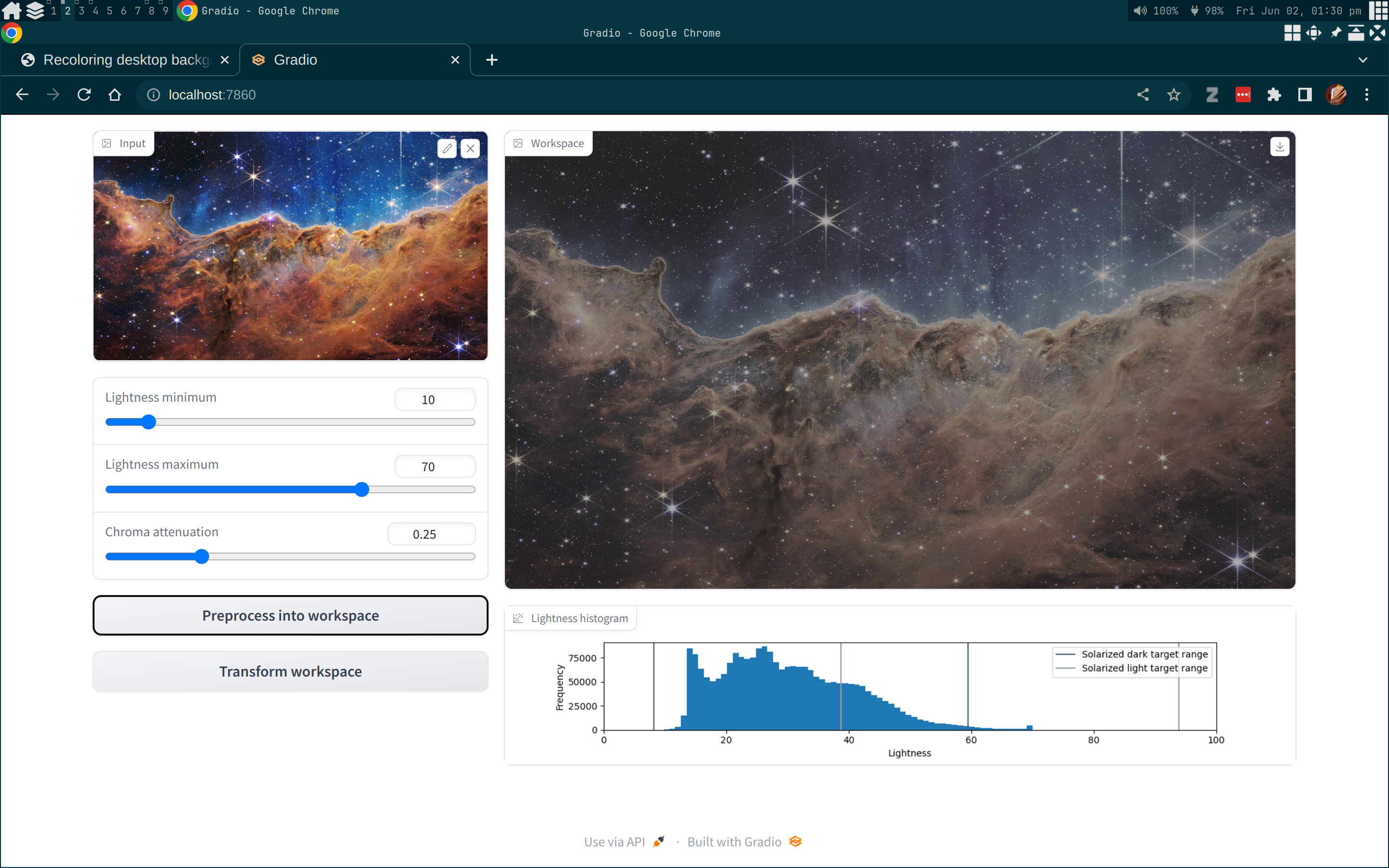
Here, we see that I had set the actual lightness range to $10 < L < 70$. After I clicked the preprocess button to perform the chroma cut and lightness remapping, we also see that the lightness histogram is acceptably in the target range for Solarized Dark. Finally, I clicked the transform button to perform the shift and rotate, yielding me the new background.
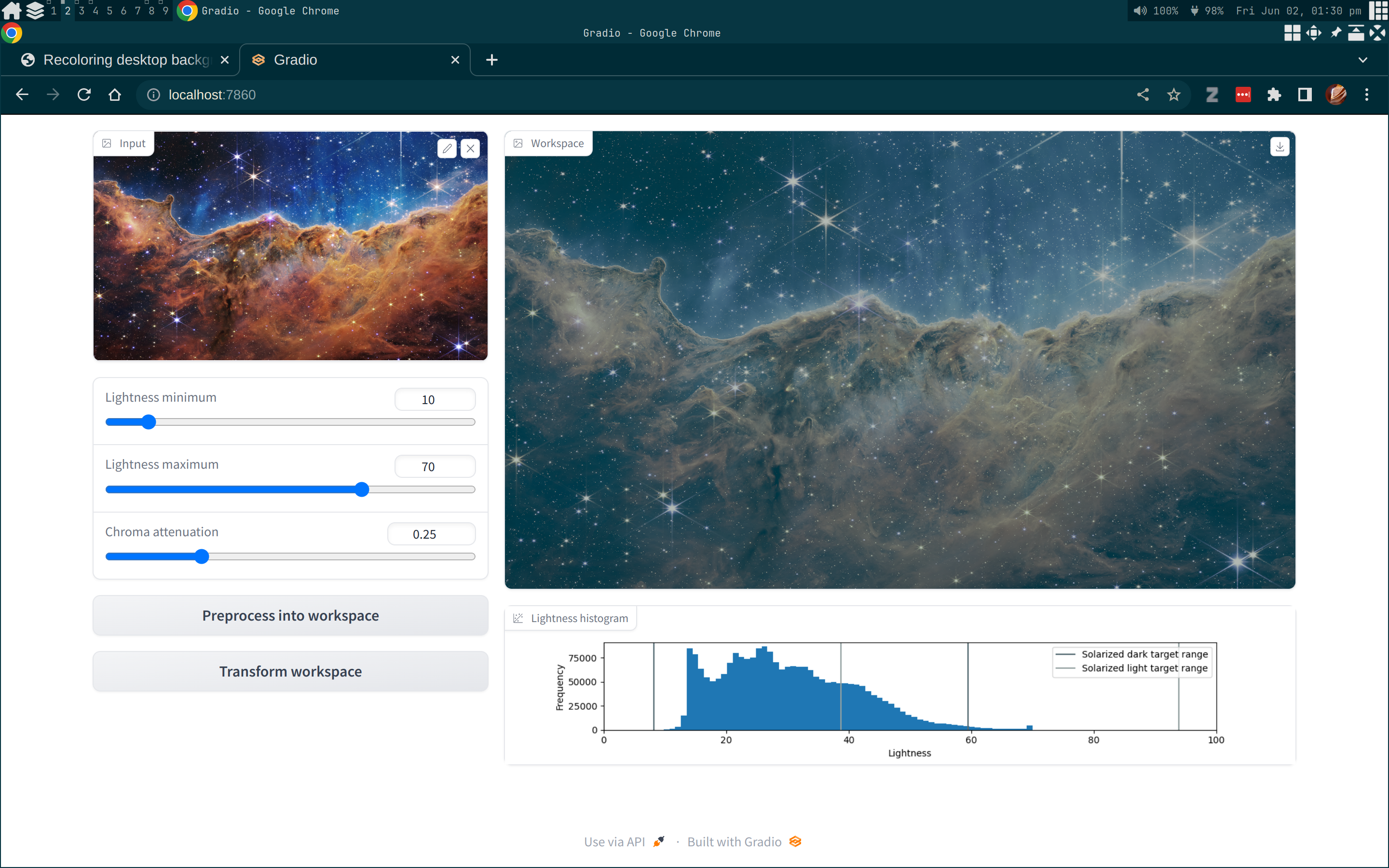
In the absence of data to base this process on, we were still successful in finding a way to align backgrounds to the Solarized base palette while also adding a bit of color to it. To do so, we chose sensible and geometric operations in CIELAB space, and we satisfied some constraints by inverting those operations to find the conditions to do so. Though this method works generally, I’ll add that there are places where change might be interesting, perhaps on the matter of defining a new style that works generally or reshaping the distribution of lightnesses. But in any case, though what I did wasn’t exactly tipping over the spinning top, I can have the wonderful colors of the Carina Cliffs back now!