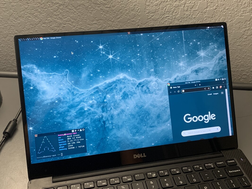
Recoloring backgrounds to align with the Solarized Dark base palette

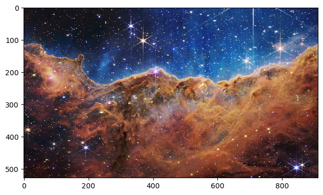
I know that I’m not the only person who made the “Carina Cliffs” into their desktop background on the day those first JWST shots were released. I had the idea shortly after I saw them, and it’s stayed on my desktop through the months since. However, I also switched from Windows to Pop!_OS to Arch Linux along the way, and sooner or later I wanted to theme my system. I eventually settled on Solarized Dark as my palette of choice, but then I had a problem. Solarized Dark focused on muted hues of blue as its base palette, but that clashed with the vibrant, orange splashes of my new favorite background.

import numpy as np
import matplotlib.pyplot as plt
from skimage import io, color

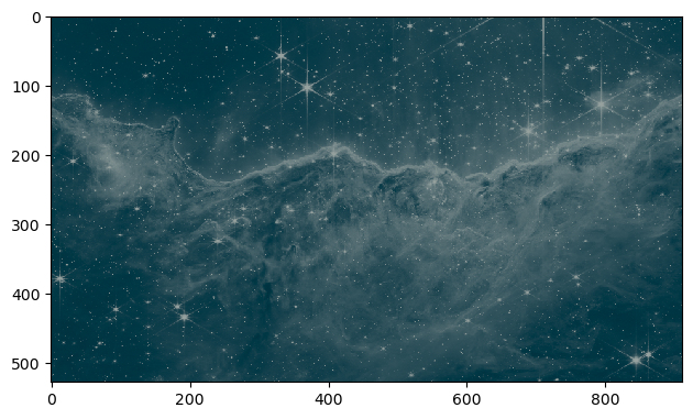
image = io.imread('carina.png')
image = image[::8, ::8] # downsample the image to 1/64 size for this blog post
io.imshow(image)
plt.show()

The ordinary idea would have been to switch to a background that aligned better, but–no–I wanted to keep my “Carina Cliffs”. So, I needed to recolor it. There were a couple of ways I could have gone about it, like composing the shot from scratch. The original infrared data was out there, but I was no color scientist.

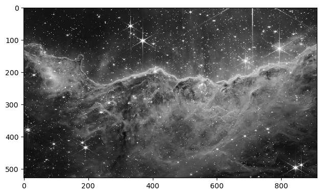
Instead, my plan started with converting the image to grayscale (though throwing out the color hurt somewhat).

image = color.rgb2gray(image)

io.imshow(image)
plt.show()

Next, I wanted to map grayscale values to colors along a “curve” going through the base palette of Solarized Dark. But what was this “curve”?

The Solarized Dark palette originally defined its colors as carefully placed points in the CIELAB space. Unlike RGB, the CIELAB space moved away from pixel brightnesses to coordinates based on human vision. Consequently, moving along any straight path in this space should look like a natural transition of colors. This is what I wanted to take advantage of by drawing a “curve”.

That said, though I knew Solarized Dark was careful about its color coordinates. I didn’t know exactly what it did. At worst, I thought that I might need to draw a Bezier curve, but it turned out to be much simpler.

# palette[:, 0] is L, palette[:, 1] is A, palette[:, 2] is B
palette = np.array([
    [ 15, -12, -12], # Base03
    [ 20, -12, -12], # Base02
    [ 45,  -7,  -7], # Base01
    [ 50,  -7,  -7], # Base00
    [ 60,  -6,  -3], # Base0
    [ 65,  -5,  -2], # Base1
    [ 92,   0,  10], # Base2
    [ 97,   0,  10], # Base3
])

mean = palette.mean(axis=0)
print('mean:', mean)

U, sigma, V = np.linalg.svd(palette-mean)
principal_component = V[0]
print('principal_component:', principal_component)

line_pts = np.outer(np.linspace(-42, 42, 10), principal_component)+mean

fig = plt.figure()
ax = plt.axes(projection='3d')
ax.scatter3D(palette[:, 0], palette[:, 1], palette[:, 2], c=palette[:, 0])
ax.plot3D(*line_pts.T)

plt.show()

mean: [55.5   -6.125 -2.875]
principal_component: [0.95104299 0.14562397 0.27260023]

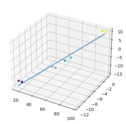
In fact, the entire base palette was placed approximately along a straight line! The “curve” I wanted could just be this line. In my searches, I found one approach to getting it: finding the “principal component” using the “SVD”. That method gave some parameters of the line that I needed.

That was:

1. mean: a reference point on the line
2. principal_component: a unit vector in the direction of the line

There was just one last thing I needed: the endpoints. This was something I just eyeballed.

t_start = -42 # approx where base03 is
t_end = 11 # approx where base1 is

print('t_start:', t_start)
print('t_end:', t_end)

# copied from previous cell
fig = plt.figure()
ax = plt.axes(projection='3d')
ax.scatter3D(palette[:, 0], palette[:, 1], palette[:, 2], c=palette[:, 0])
ax.plot3D(*line_pts.T)

# plot the endpoints of the line
ax.plot3D(*(principal_component*t_start+mean).T, 'x', color='blue')
ax.plot3D(*(principal_component*t_end+mean).T, 'x', color='blue')

plt.show()

t_start: -42
t_end: 11

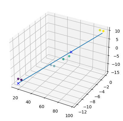
These endpoints were represented as the final parameters:

1. t_start: zero brightness will be mapped to principal_component*t_start+mean
2. t_end: max brightness will be mapped to principal_component*t_end+mean

And with this line fully defined, I could hop to it from grayscale as I planned.

orig_shape = image.shape
image = image.flatten()
image = image*(t_end-t_start)+t_start
image = np.outer(image, principal_component)+mean
image = image.reshape(*orig_shape, 3)
image = color.lab2rgb(image)

io.imshow(image)
plt.show()

And so, I had my new “Carina Cliffs”, recolored to align with my new theme! I’m sure that this isn’t the only method, but it was the first one that I tried and liked.

If anyone else wants to recolor their backgrounds in this way, it turns out to be quite the churn. For an 8K background like the “Carina Cliffs”, I’ve had a couple of OOM-kills along the way on my 8GB machine, but I have optimized the process into this quick and small script.