Investigating the math of waveshapers: Chebyshev polynomials
Over a year ago, I wrote “Adding harmonic distortions with Arduino Teensy”. In that post, I happened upon a way to apply any arbitrary profile of harmonics using a Teensy-based waveshaper (just except that waveshapers categorically can’t vary the phase of each harmonic). However, when I wrote that, I totally missed out on the established literature on the topic! Even in 1979, there was “A Tutorial on Non-Linear Distortion or Waveshaping Synthesis”, and I ultimately had taken a very convoluted path only to arrive at the same place!
To compare it to the method I showed before, one can adapt that 1979 tutorial to the Teensy waveshaper quite naturally, and the adapted method is far easier to implement and more concise. However, to do the adaptation, we have to know one thing: what is a “Chebyshev polynomial”?
Chebyshev polynomials can be used in a rigorous approach to building waveshapers according to some desired profile of harmonics. In this context, their claim to fame is that they’re polynomials that can twist a $\cos x$ wave into its $n$-th harmonic, or in other words
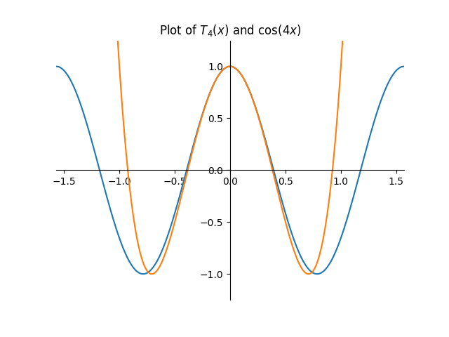
\[T_n(\cos x) = \cos(nx)\]You already know one if you can recall the double-angle formula, $\cos(2x) = 2\cos^2 x - 1$. Now, imagine un-substituting $\cos x$ from the right-hand side, and you’ll get the Chebyshev polynomial $T_2(x) = 2x^2 - 1$. Then, imagine a double-double-angle formula, $\cos(4x) = 2\cos^2(2x)-1$, and expand that to $8\cos^4 x - 8\cos^2 x + 1$. Unsubstituting $\cos x$ from that gets the Chebyshev polynomial $T_4(x) = 8x^4 - 8x^2 + 1$.
Now, algebraically manipulating these angle identities into polynomials is a nice hat trick, but there is a simpler way to think of all the Chebyshev polynomials. In the first section of Chebyshev Polynomials by Mason and Handscomb (the first book that appeared on Google Scholar, don’t @ me), you can find the claim that algebraic manipulations of De Moivre’s theorem are—technically—all that you need to find a Chebyshev polynomial $T_n(x)$ for arbitrary $n$. But in that same section, you can find an easy recurrence that connects them all:
\[T_n(x) = 2x T_{n-1}(x) - T_{n-2}(x)\]where $T_0(x) = 1$ and $T_1(x) = x$ to start. For example, we can use this recurrence to get from $T_2(x)$ to $T_4(x)$ by way of $T_3(x)$
\[\begin{align*} T_3(x) & = 2x T_2(x) - T_1(x) \\ & = 2x (2x^2-1)-x \\ & = 4x^3 - 3x \end{align*}\] \[\begin{align*} T_4(x) & = 2x T_3(x) - T_2(x) \\ & = 2x (4x^3-3x)-(2x^2-1) \\ & = 8x^4 - 6x^2 - 2x^2 + 1 \\ & = 8x^4-8x^2+1 \end{align*}\]where you can notice here that $T_3(x)$ corresponds with the triple-angle formula!
Hopefully, that’s enough about Chebyshev polynomials for us to start understanding how to use them here. Assume that $\cos x$ is our input signal (we can see how this assumption breaks down later). By the definition of the Chebyshev polynomials, $\cos x$ happens to be equal to $T_1(\cos x)$, and so we can therefore use $T_1(x) = x$ as a kind of stand-in for $\cos x$. In the same way, we can represent some $n$-th harmonic as the polynomial $T_n(x)$. Therefore, some linear combination of $\cos x$ and its harmonics can be represented as a linear combination of the Chebyshev polynomials, and that would be another polynomial in itself!
In other words, if we let $\alpha_n$ be the ratios between the harmonic and the fundamental (for $n \geq 2$, since $n = 1$ is the fundamental itself), then this polynomial can be written as
\[f(x) = T_1(x) + \sum_{n=2}^\infty \alpha_n T_n(x)\]In fact, this is only a few minor tweaks away from being what we throw into the lookup table of a Teensy waveshaper. Everything can be written in only four steps!
How to generate a waveshaper lookup table in four steps!
-
Decide what amplitude ratios $\alpha_n$ each $n$-th harmonic should have with the fundamental frequency
-
Build a preliminary function $f_0(x)$ as the linear combination of the Chebyshev polynomials
\[f_0(x) = T_1(x) + \sum_{n=2}^\infty \alpha_n T_n(x)\]where the first Chebyshev polynomials are
\[\begin{align*} T_0(x) & = 1 \\ T_1(x) & = x \\ T_2(x) & = 2x^2-1 \\ T_3(x) & = 4x^3-3x \\ T_4(x) & = 8x^4-8x^2+1 \end{align*}\]and the rest can be derived by the recurrence relation
\[T_{n+1}(x) = 2 x T_n(x)-T_{n-1}(x)\] -
Shift $f_0(x)$ so that it maps zero to zero (for preventing constant DC) by evaluating $f_0(x)$ at $x=0$ then subtracting that
\[f_1(x) = f_0(x)-f_0(0)\] -
Normalize $f_1(x)$ by finding the maximum absolute value for $-1 < x < 1$ (try plotting $f_1(x)$) then dividing by that
\[f_2(x) = \frac{f_1(x)}{f_{\text{1,maxabs}}}\]
The above function, $f_2(x)$, is your final function. Evaluate it at as many points within $-1 < x < 1$ as can fit in your waveshaper’s LUT! If the input sine wave swings exactly within $-1 < x < 1$, then the ratios $\alpha_n$ will be realized. Otherwise, different and smaller ratios will occur.
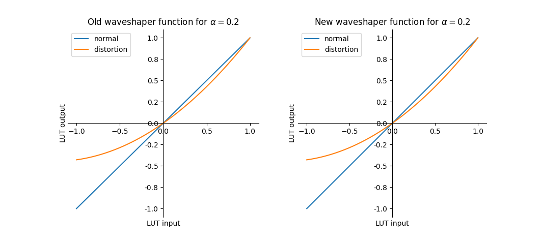
Using this method, I can perfectly replicate my old post!
-
In that old post, I chose to give the second harmonic a weight of $0.2$ and no weight to the higher ones, so $\alpha_2 = 0.2$ and $\alpha_n = 0$ for $n > 2$.
-
The sum reduces to a single Chebyshev polynomial term, so the preliminary function is
\[f_0(x) = x + 0.2 (2x^2-1)\] -
We can calculate that $f_0(0)=-0.2$, so our new function must be
\[f_1(x) = x+0.2 (2x^2-1)+0.2\] -
Plotting $f_1(x)$ reveals that it achieves a maximum absolute value of 1.4 at $x=1$, so our final function must be
\[f_2(x) = \frac{x+0.2 \cdot (2x^2-1)+0.2}{1.4}\]
That function simplifies to $\frac{2}{7}x^2+\frac{5}{7}x$.
We’ve essentially reached parity with my last blog post, but one question remains: what happened to all the phase shifts I had done? In fact, if I used the $\cos x$ wave and not the $\sin x$ wave as my basis, I could have avoided that altogether. While Chebyshev polynomials do what’s written on their tin when passed $\cos x$ as the input, you can show that it doesn’t do the same for $\sin x$ waves:
\[\begin{align*} T_n(\sin x) & = T_n \big(\cos(x - \frac{\pi}{2}) \big) \\ & = \cos\big(n(x-\frac{\pi}{2})\big) \\ & = \cos(nx - n\frac{\pi}{2}) \\ & = \sin(nx-n\frac{\pi}{2}+\frac{\pi}{2}) \\ & = \sin\big(nx-(n-1)\frac{\pi}{2}\big)\end{align*}\]And hence came the phase shifts.
Finally, let’s address the assumption that we made from the start: that our input was a $\cos x$ wave. We’ve seen now that even trying $\sin x$ waves instead already breaks the result. That is, only when we give one specific sinusoid, $\cos x$, will we get all the harmonics back with no phase shifts. Another way we can break this is to give it a wave of some varying amplitude $a(t) \leq 1$ (i.e. an ADSR envelope) or even an arbitrary input. In that case, I don’t know where the impacts end. At the very least, I can address one of them: constant DC shifts.
For $a(t) = 0$, a waveshaper will see nothing but zero, and it may decide to map that to something nonzero. This is because Chebyshev polynomials weren’t defined with that in mind either. For example, $T_2(0)=-1$. If my headphones saw -1 volts at DC, they’d blow. From my old post, I had only seen that happen when I added even harmonics, and I had seen that adding a constant equal to $\alpha_n$ or $-\alpha_n$ would correct that. Ultimately though, the easiest way to correct this effect is to just evaluate the waveshaper function at $x=0$, then subtract that value. That’s step 3.