Rebuilding ESP32-fluid-simulation: the pressure projection step of the sim task (Part 5)
It’s been a while since my last post, but let’s bring this series to its finale. Out of all the parts of the fluid sim, the last piece I have not explained is the pressure projection. The code alone doesn’t reveal the great deal of context that goes into its design. Here’s a hint: it’s actually a linear algebra routine involving a “sparse matrix”. Though it’s possible these days to implement the pressure projection without needing to know all that context, thanks to articles like Jamie Wong’s post, the GPU Gems chapter, and Stam’s “Real-Time Fluid Dynamics for Games”, achieving a believable fluid simulation on an ESP32 would have been impossible. I’ve personally tried it before, and after knowing? All I needed was to switch in a technically superior method. There was a reason why I dedicated airtime to this—let me explain.
In Part 3, I covered the Navier-Stokes equations, and in part 4, we covered how parts of the equations were discretized differently. Well, to begin with I need to cover one last thing that involves continuous fields and not discrete arrays: the “Helmholtz-Hodge decomposition”.
It’s mentioned in the GPU Gems chapter, and for that Stam’s 1999 “Stable Fluids” paper is cited. In the end, I had found “Stable Fluids” to be the definitive place to start looking for context, and there I borrow much of my understanding. Now, it itself cites a section of the book A mathematical introduction to fluid mechanics by Chorin and Marsden. Building upon this section, I’ll get into what the “Helmholtz-Hodge decomposition” is. Though, I won’t get into why it is i.e. all of the book preceding that section. That’s outside the scope I want to take here, but that’s also outside what I can comfortably do—I’ll admit. With that said, what is it, and how do we apply it?
We can derive the pressure projection from the decomposition. To begin, the decomposition itself is this: given some vector field $\bold{w}$ that is defined over a bounded space, it can be taken as the following sum
\[\bold{w} = \bold{v} + \nabla p\]where $\nabla p$ is the gradient of a scalar field which we can solve for—I’ll explain shortly—and $\bold v$ is a vector field that has zero divergence and zero flow across the boundary. Now, let $\bold w$ be the uncorrected velocity field. We need to satisfy the incompressibility constraint, which is that the field has zero divergence, and now it just so happens that $\bold v$ is the zero-divergence part of $\bold w$. We just need to isolate $\bold v$!
\[\bold{v} = \bold{w} - \nabla p\]That’s how we want to apply Helmholtz-Hodge decomposition, but we need more before we have a concrete routine in our hands. Before we can subtract $\nabla p$ from $\bold w$, we need to find what $p$ is in the first place! Therein lies the meat of the pressure projection.
Also in the Chorin and Marsden section, you’d find that the proof of the Helmholtz-Hodge decomposition builds upon the pressure being the solution to a particular “boundary value problem”, one that Stam noted to involve a case of “Poisson’s equation”. In a “boundary value problem”, we’re given a bounded space as a domain, the governing differential equations that a function on that space must satisfy, and the values that the function (and/or values of that function’s derivative) must take on the boundary i.e. the “boundary conditions”.
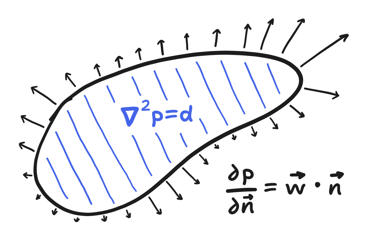
Regarding “Poisson’s equation”, I’m not qualified to opine about it or anything, so I’ll just say that it’s a partial differential equation where one scalar field is equal to the Laplacian of another scalar field. If there’s an intuitive meaning to it, that’s currently lost on me.
Anyway, the boundary value problem is this: given $\bold{w}$, $p$ should satisfy the following case of Poisson’s equation
\[\nabla^2 p = \nabla \cdot \bold{w}\]on the domain, whereas on the boundary its “directional derivative” is specified.
When I say “directional derivative”, I’d like you to recall that explanation of the partial derivative I did in Part 3, where I mentioned that $\frac{\partial p}{\partial x}$ and $\frac{\partial p}{\partial y}$ were just the slopes of two lines in the many that make up the plane tangent to the field. The “directional derivative” is the slope of a potentially different line, the one running in the direction that the derivative is being taken with respect to.
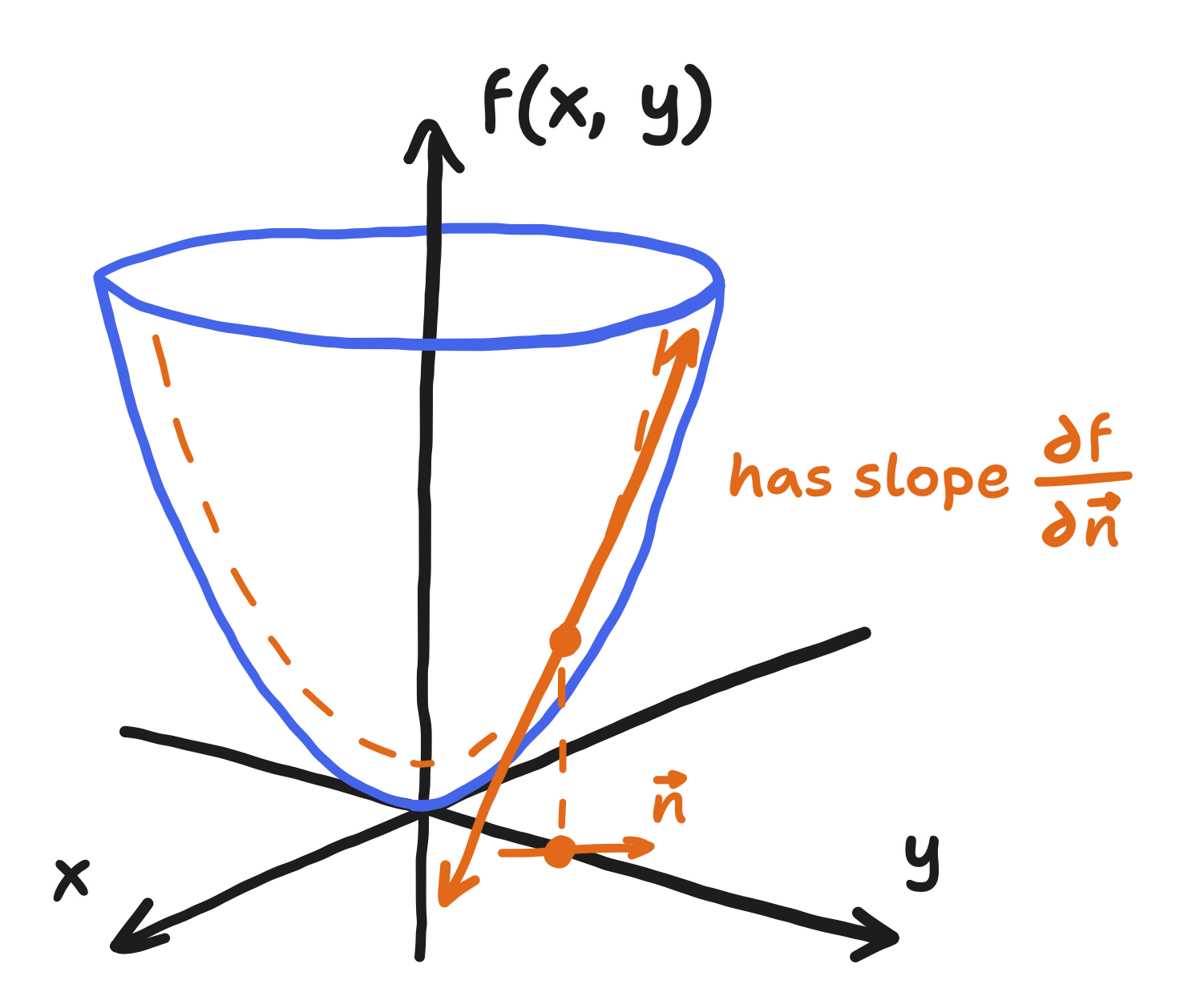
In this case, the directional derivative with respect to the normal (the direction perpendicular to the boundary and pointing outwards) is equal to the component of $\bold{w}$ that is in that direction. A specification of the derivative, not the value, of $p$ like this is said to be a “Neumann” boundary condition.
\[\frac{\partial p}{\partial \bold{n}} = \bold{w} \cdot \bold{n}\]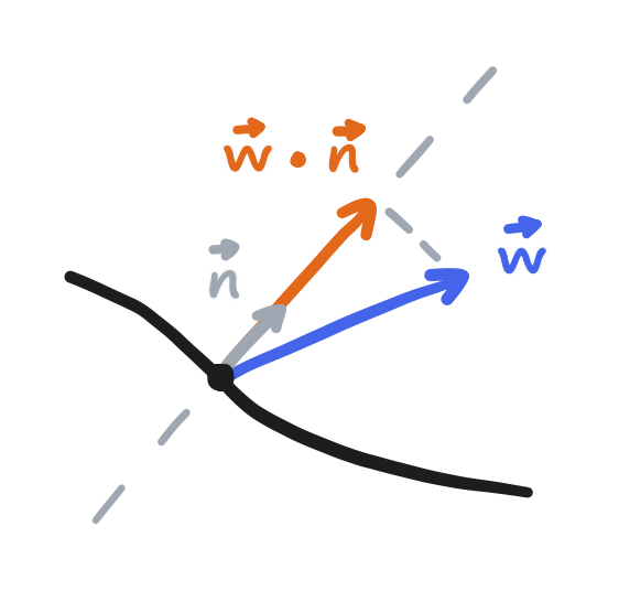
There are many ways to solve this, but we’ll start by again turning to discretization with a grid. This time, though, it’ll be an entire finite difference method.
Review: The finite difference discretization
I mentioned them in passing in Part 4, but you may or may not be familiar with the finite difference approximation of a derivative. A “finite difference” can be taken quite literally: it’s the “difference” i.e. subtraction between the values of a function at points separated by a “finite” i.e. not infinitesimal distance. It’s what happens when you don’t take the limit inside the definition of the derivative.
\[\frac{df}{dx} = \lim_{h \to \infty} \frac{f(x) - f(x-h)}{h} \approx \frac{f(x) - f(x-\Delta x)}{\Delta x}\]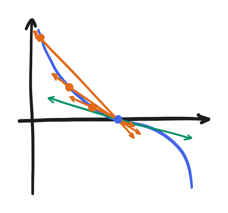
In general, there are many different ways to approximate the derivative using a linear combination of different sets of neighboring points. Anyway, that’s out of scope. We should focus on the common cases. The above expression shows the “backward” difference, taking a point and its preceding point. The other two common cases are the “forward” difference and the “central” difference.
The forward difference uses a point and its succeeding point,
\[\frac{df}{dx} \approx \frac{f(x + \Delta x) - f(x)}{\Delta x}\]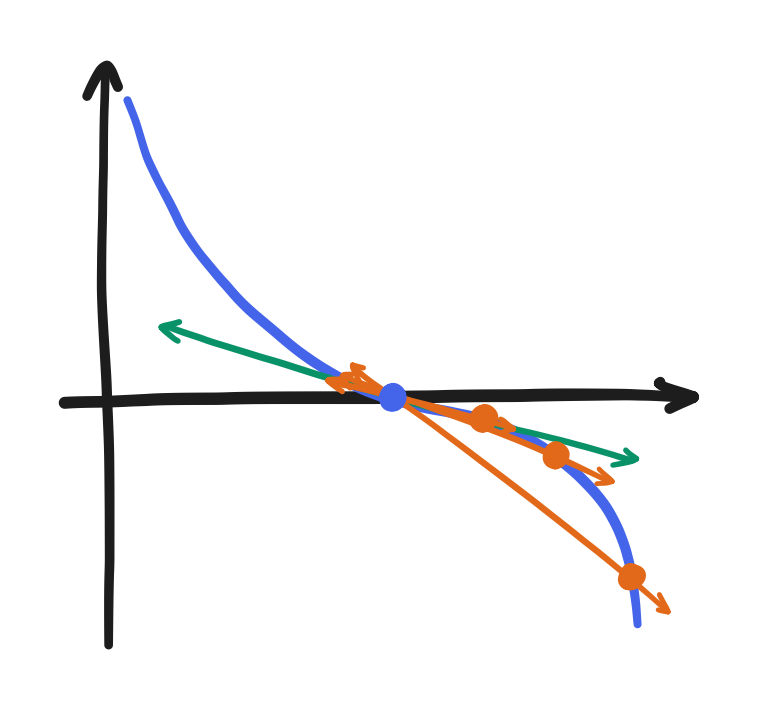
and the central difference uses the preceding point and the succeeding point.
\[\frac{df}{dx} \approx \frac{f(x + \Delta x) - f(x - \Delta x)}{2 \Delta x}\]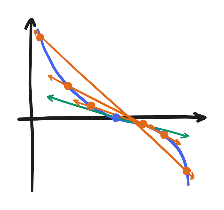
All of these expressions converge on the same value as $\Delta x$ shrinks, but we’ll end up using the central difference the most. That said, the forward and backward differences also get involved in today’s scheme.
Anyway, because we discretized the fields with grids, this approximation is useful to us. First, extending this idea to partial derivatives is quite simple! Recall that it’s the derivative of a field with respect to one component while keeping all others constant. Because we discretized space with a grid, all points have left, right, top, and bottom neighbors (all besides the ones on the boundary, but we’ll get to them at some point). So, we can use the “forward” and “backward” neighbors in each direction, $\frac{\partial f}{\partial x}$ using the left and right and $\frac{\partial f}{\partial y}$ using the top and bottom.
\[\frac{\partial f}{\partial x} \approx \frac{f(x + \Delta x, y) - f(x - \Delta x, y)}{2 \Delta x}\] \[\frac{\partial f}{\partial y} \approx \frac{f(x, y + \Delta y) - f(x, y - \Delta y)}{2 \Delta y}\]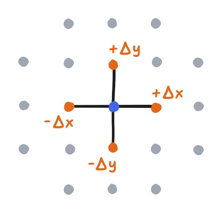
Finally, recall that a field that’s discretized with a grid can be replaced with an array, and so we can rewrite the above central differences using indices.
\[g_x[i, j] = \frac{f[i+1, j] - f[i-1, j]}{2 \Delta x}\] \[g_y[i, j] = \frac{f[i, j+1] - f[i, j-1]}{2 \Delta y}\]With this, approximating the differential operators is as easy as taking their definitions and replacing each partial derivative with its finite difference counterpart. Let’s write out the ones we’ll use for the rest of this article.
Discretizing the gradient and the divergence with the central differences gets the following:
\[\nabla f = \begin{bmatrix} \displaystyle \frac{\partial f}{\partial x} \\[1em] \displaystyle \frac{\partial f}{\partial y} \end{bmatrix} \approx \begin{bmatrix} \displaystyle \frac{f[i+1, j] - f[i-1, j]}{2 \Delta x} \\[1em] \displaystyle \frac{f[i, j+1] - f[i, j-1]}{2 \Delta y} \end{bmatrix}\] \[\nabla \cdot \bold{f} = \frac{\partial f_x}{\partial x} + \frac{\partial f_y}{\partial y} \approx \frac{f[i+1, j] - f[i-1, j]}{2 \Delta x} + \frac{f[i, j+1] - f[i, j-1]}{2 \Delta y}\]That leaves the Laplacian. There happens to be a “but actually” to discuss here. You may recall from Part 3 that the Laplacian is the divergence of the gradient but also that it can be written as a sum of the second partial (non-mixed) derivatives.
\[\nabla^2 f \equiv \nabla \cdot (\nabla f) = \frac{\partial^2 \! f}{\partial x^2} + \frac{\partial^2 \! f}{\partial y^2}\]One possible discrete approximation—one that uses what we’ve already mentioned—is to take the discrete gradient and then take the discrete divergence. Instead, the typical thing to do builds upon the latter definition. A second derivative can itself be approximated with finite differences, and the central difference way to do it is this:
\[\frac{d^2 \! f}{d x^2} \approx \frac{f(x+\Delta x) - 2f(x) + f(x - \Delta x)}{\Delta x^2}\]After extending this approximation to the partial derivative and rewriting it in terms of array values, that latter definition becomes the following.
\[\frac{\partial^2 \! f}{\partial x^2} + \frac{\partial^2 \! f}{\partial y^2} \approx \frac{f[i+1, j] - 2 f[i,j] + f[i-1, j]}{\Delta x^2} + \frac{f[i, j+1] - 2 f[i, j] + f[i, j-1]}{\Delta y^2}\]Finally, if the grid is square—that is, $\Delta x = \Delta y$—then the $f[i,j]$ terms can be combined cleanly, and it just reduces to this:
\[\frac{\partial^2 \! f}{\partial x^2} + \frac{\partial^2 \! f}{\partial y^2} \approx \frac{f[i+1,j] + f[i-1,j] + f[i, j+1] + f[i, j-1] - 4 f[i, j]}{\Delta x^2}\]This is how the Laplacian is typically discretized, but it’s actually not equal to the discrete divergence of the discrete gradient. Going about it that way happens to get you the above but with $\Delta x$ and $\Delta y$ being twice as large and the neighbor’s neighbor being used (two to the left, two to the right, etc). And, for the record, it didn’t look that good when I tried it.
Really, it goes to show that the “Stable Fluids” discretization will be simple but not very faithful to the original boundary value problem. Once before, years ago, I didn’t realize it could be flawed, and I lost many hours because of that. On another note, I reached out a year ago to Stam about it, and he mentioned that he instead used the “marker-and-cell (MAC) method” in his past professional work on Maya (now Autodesk Maya) and I managed to work out after that the MAC method does happen to make the two equal.
Anyway, that’s the finite difference discretization (or, well, a simple case of it) and how it is applied to the gradient, divergence, and Laplacian. It’s a fundamental concept to grasp because—as you will see—a discrete approximation of differential operators can turn our boundary value problem into something we can solve.
So, how do we use finite differences to solve the problem? At this point, the “Stable Fluids” paper goes on to use a different technique altogether, so instead we can turn to the methods you can find in Stam’s “Real-time Fluid Dynamics for Games” or the GPU Gems chapter. I’ll take the time to emphasize some of the context, though.
To begin with, we need to apply the finite difference discretization to the boundary value problem. I’ll say here that we need to treat both the governing equation and the boundary conditions here and now.
The governing equation, our Poisson, is simple enough; we just replace the Laplacian and the divergence with their discrete counterparts. In those articles, the central difference version is used, so that’s what we’ll use here. Furthermore, the pressure field is the unknown here, not the uncorrected velocity field, so it makes sense to calculate the divergence once and hold the result as a temporary scalar field. Finally, there’s no reason to not use a square grid. Overall, Poisson’s equation becomes this:
\[\frac{p[i+1, j] + p[i-1, j] + p[i, j+1] + p[i, j-1] - 4 p[i, j]}{\Delta x^2} = d[i, j]\]where the temporary $d[i, j]$ holds the discrete divergence of $\bold{w}$
\[d[i,j] = \frac{w_x[i+1, j] + w_x[i-1, j] + w_y[i, j+1] + w_y[i, j-1]}{2 \Delta x}\]Notice here that $\bold{w}$, whose divergence was replaced with $d$, doesn’t directly appear in the governing equation anymore. Also notice here that discretizing the Poisson equation does not give us one single unknown to isolate. Given some $i$ and $j$, there’s five unknowns and one known, and that’s not solvable.
Before we deal with that, the boundary conditions is the other half we need to discretize. You may have noticed a plot hole here already: there isn’t always a left, up, right, or down neighbor. $p[i-1, j]$ doesn’t exist if $i = 0$. Now, remember how we used ghost points to complete the bilinear interpolation at the boundary? I’ll show that we can discretize our Neumann condition with the same ghost points, and in doing so we’ll find out what to do here.
I do have to preface this with something real quick, though. I mentioned that the directional derivative of $\bold w$ with respect to the normal is equal to the component of $\bold w$ in that direction, as was said in the Chorin and Marsden section. In Stam’s “Stable Fluids” and the GPU Gems article, the same boundary value problem is presented but with the directional derivative being equal to zero. It’s a clear discrepancy. Now, I’ll have to ask you to switch with me to Stam’s definition. This sounds arbitrary, but I promise to give an explanation that might bridge the gap in a moment.
That out of the way, our boundary condition just manifests as setting $\frac{\partial p}{\partial x}$ or $\frac{\partial p}{\partial y}$ because the domain is rectangular. Let’s see what to do on the top side first. There, the normal direction the $+y$-direction. That is, $\frac{\partial p}{\partial \bold{n}} = 0$ manifests as $\frac{\partial p}{\partial y} = 0$. We then replace $\frac{\partial p}{\partial y}$ with its finite difference counterpart, but there’s a twist. The forward difference, not the central difference, is used. That gets us the following.
\[\frac{p[i, N] - p[i, N-1]}{\Delta x} = 0\]where $i$ is any horizontal index, $N-1$ is the vertical index of the last real row, and $N$ is the vertical index of the ghost row. The implication of this statement is obvious: the ghost row must take on the values of the real row.
\[p[i, N] = p[i, N-1]\]The same conclusion should be expected for all sides. For the bottom side, it’s reached by applying the backward difference on $\frac{\partial p}{\partial y} = 0$. For the right side, the forward difference on $\frac{\partial p}{\partial x} = 0$. For the left, the backward difference on $\frac{\partial p}{\partial x} = 0$. It should sound quite similar to what we did for the bilinear interpolation, though back then the ghost row had to take on the negative.
And now, with all this in mind, I think I can explain the discrepancy: it comes from grid choice. Remember from Part 4 that the boundary is supposed to simulate a wall that runs between the last real row and the ghost row? That was accomplished by making the ghost rows and columns take the negative because that makes the value of the bilinear interpolation at the “wall” equal to zero by definition. If $\bold{w}$ at the boundary is zero, then $\bold{w} \cdot \bold{n}$ must be zero. If $\bold{w} \cdot \bold{n}$ is zero, then even when following the definition from Chorin and Marsden, $\frac{\partial p}{\partial \bold{n}}$ must be zero. Though, I’m a mere fluid sim amateur, and I’m not sure if this explanation is acceptable.
One last aside! Though it may sound strange that we switched from applying the central difference to the forward difference, I think we can imagine together what it would imply if we kept it: at the top boundary, the central difference must be equal to zero
\[\frac{p[i, N] - p[i, N-2]}{\Delta x} = 0\]and therefore the ghost row should take on the values of the second-to-last row.
\[p[i, N] = p[i, N-2]\]That conclusion doesn’t sound as natural.
That completes the finite difference version of our boundary value problem! That leaves solving it, and that can be done with a computer. Now, there’s that, and there’s solving it with an ESP32 for the computer. If my goal was to explain the former, then quoting my sources would’ve been effective enough, but here’s comes the necessary context.
For one, didn’t I say this involved “sparse matrices”? Here they are.
Review: Sparse matrices
You may or may not be familiar with “sparse matrices”. If you are, then you would know that they enable a great deal of optimization on a computer—to a point where even the big-O complexity is lower—without changing any of the linear algebra stuff. With such drastic improvement for free on the table, “sparse matrices” are an essential topic. And that’s all for, well, “sparse matrices” just being matrices with a lot of zeroes.
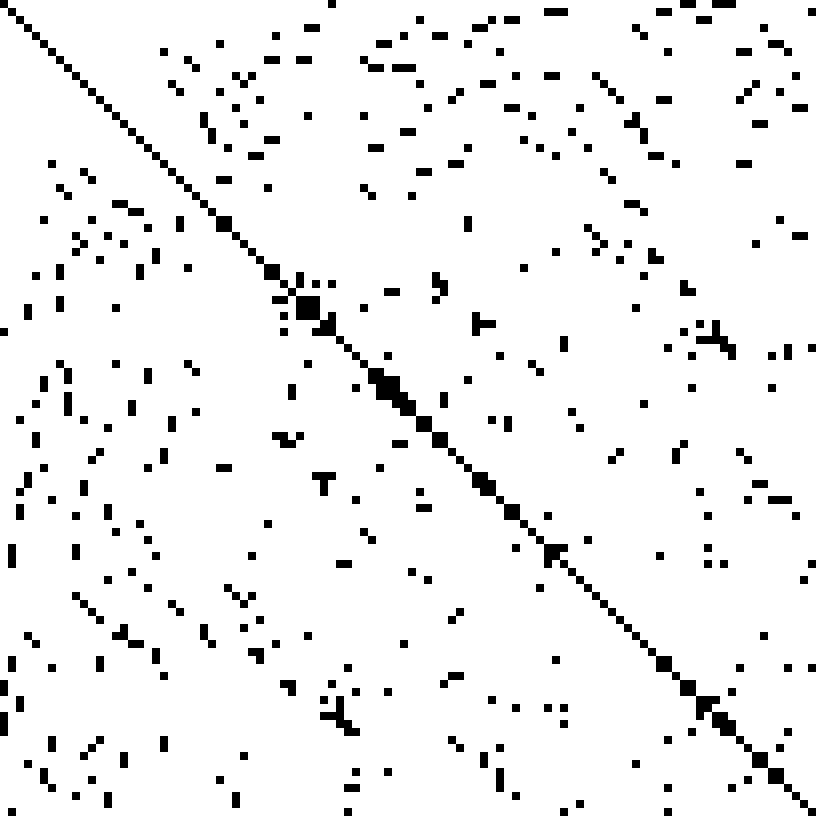
At risk of being vague about it, I’ll say that zero can be effectively implemented by doing nothing or storing nothing. Conversely, actual computation and memory is focused on the non-zero elements.
Now, speaking at length about sparse matrices is beyond me and beyond the scope of this post, but we’ll now get into our specific application of them.
I mentioned in the last part that it is more useful to think of fields—which are arrays when discretized—as very long vectors. Where was I going with that, exactly? Our arrays are a 2D arrangement of data, with each position of each element neatly corresponding to a 2D location. Now, we care less for this correspondence when we’re doing the linear algebra. Vectors are a 1D arrangement of data. To rearrange the array into a vector, convention tells us to read out the data like a book, increasing in i from left to right, then increasing in j from… bottom to top, actually, to stay in the Cartesian perspective. Once again, I already discussed the difference between matrix indexing and Cartesian indexing in Part 3. And of course, the conventional mapping isn’t the only mapping, and we’ll get to another mapping in this article eventually, but I’ve rambled enough about convention—in this section and in Part 3.
Let’s make this concrete with an example. Consider a three-by-three grid and some scalar field $x$. Then, the discretization of $x$ on that grid is a three-by-three array. Reading out its elements gets a nine-element vector. All that is depicted below.
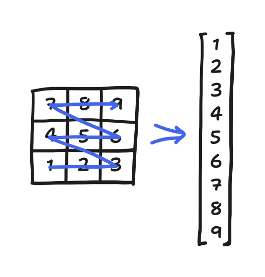
Let’s look at points 5 and 8. They’re right next to each other in 2D space, but now they’re so far apart on the vector! Such things happen with the mapping.
More importantly, with arrays rearranged as vectors, we can show that our boundary value problem, when discretized the way we’ve done it, is a classic $Ax = b$ problem! If we let $x$ be the pressure vector and $b$ be the divergence, then the $i$-th row of $A$ represents the equation for some specific point with location $i,\; j$ (yes, unfortunately $i$ and $j$ have double-meanings in this post), relating the $i$-th element of the divergence vector to the $i$-th plus four more elements of the pressure vector, one for each neighbor. For the points along the boundary, that’s only four or three elements since an element in the ghost row or column just takes the value of an actual neighbor. Furthermore, because the discretized Poisson just relates the five (or less) elements of the pressure vector, all of the elements of that row besides the five (or less) must be zero. $A$ is sparse!
Let’s apply this to our three-by-three example, and let’s do it by looking at one row at a time. First, the center element $i=1,\;j=1$ is the only element with all-real neighbors, so it stands for the typical case where the boundary conditions don’t apply. We can fill in the corresponding row of $A$ like this:
\[\frac{1}{\Delta x^2} \begin{bmatrix} \\ \\ \\ \\ 0 & 1 & 0 & 1 & -4 & 1 & 0 & 1 & 0 \\ \\ \\ \\ \! \end{bmatrix} \begin{bmatrix} p_{0, 0} \\ p_{1, 0} \\ p_{2, 0} \\ p_{0, 1} \\ p_{1, 1} \\ p_{2, 1} \\ p_{0, 2} \\ p_{1, 2} \\ p_{2, 2} \end{bmatrix} = \begin{bmatrix} d_{0, 0} \\ d_{1, 0} \\ d_{2, 0} \\ d_{0, 1} \\ d_{1, 1} \\ d_{2, 1} \\ d_{0, 2} \\ d_{1, 2} \\ d_{2, 2} \end{bmatrix}\]In this row, the element corresponding to $i=1,\;j=1$ itself gets a $-4$, the ones corresponding to its neighbors get a $1$, and all other elements get a zero. And I’d be much obliged if you could confirm for yourself that this row-vector product gets back our discretized Poisson’s equation.
Now, one step to the left lands us on $i = 0,\;j = 1$, which is on the left boundary, so applying our discretized Neumann boundary condition gets us this equation
\[\frac{p[i+1, j] + p[i, j+1] + p[i, j-1] - 3 p[i, j]}{\Delta x^2} = d[i, j]\]where the terms canceling gets us this $-3$ instead of a $-4$. It’s corresponding row in $A$ looks like this:
\[\frac{1}{\Delta x^2} \begin{bmatrix} \\ \\ \\ 1 & 0 & 0 & -3 & 1 & 0 & 1 & 0 & 0 \\ 0 & 1 & 0 & 1 & -4 & 1 & 0 & 1 & 0 \\ \\ \\ \\ \! \end{bmatrix} \begin{bmatrix} p_{0, 0} \\ p_{1, 0} \\ p_{2, 0} \\ p_{0, 1} \\ p_{1, 1} \\ p_{2, 1} \\ p_{0, 2} \\ p_{1, 2} \\ p_{2, 2} \end{bmatrix} = \begin{bmatrix} d_{0, 0} \\ d_{1, 0} \\ d_{2, 0} \\ d_{0, 1} \\ d_{1, 1} \\ d_{2, 1} \\ d_{0, 2} \\ d_{1, 2} \\ d_{2, 2} \end{bmatrix}\]Another step down lands up on $i = 0, \; j = 2$, which is on both the left and top boundary, and that gets us the following equation,
\[\frac{p[i+1, j] + p[i, j+1] - 2 p[i, j]}{\Delta x^2} = d[i, j]\]and its corresponding row looks like this.
\[\frac{1}{\Delta x^2} \begin{bmatrix} \\ \\ \\ 1 & 0 & 0 & -3 & 1 & 0 & 1 & 0 & 0 \\ 0 & 1 & 0 & 1 & -4 & 1 & 0 & 1 & 0 \\ \\ 0 & 0 & 0 & 1 & 0 & 0 & -2 & 1 & 0 \\ \\ \! \end{bmatrix} \begin{bmatrix} p_{0, 0} \\ p_{1, 0} \\ p_{2, 0} \\ p_{0, 1} \\ p_{1, 1} \\ p_{2, 1} \\ p_{0, 2} \\ p_{1, 2} \\ p_{2, 2} \end{bmatrix} = \begin{bmatrix} d_{0, 0} \\ d_{1, 0} \\ d_{2, 0} \\ d_{0, 1} \\ d_{1, 1} \\ d_{2, 1} \\ d_{0, 2} \\ d_{1, 2} \\ d_{2, 2} \end{bmatrix}\]All of the possibilities—in the three-by-three example or in any size of screen—is covered by these cases after adjusting for whichever neighbors are in a ghost row/column. Let’s fill in the rest of $A$.
\[\frac{1}{\Delta x^2} \begin{bmatrix} -2 & 1 & 0 & 1 \\ 1 & -3 & 1 & 0 & 1 \\ 0 & 1 & -2 & 0 & 0 & 1 \\ 1 & 0 & 0 & -3 & 1 & 0 & 1 \\ & 1 & 0 & 1 & -4 & 1 & 0 & 1 \\ & & 1 & 0 & 1 & -3 & 0 & 0 & 1 \\ & & & 1 & 0 & 0 & -2 & 1 & 0 \\ & & & & 1 & 0 & 1 & -3 & 1 \\ & & & & & 1 & 0 & 1 & -2 \end{bmatrix} \begin{bmatrix} p_{0, 0} \\ p_{1, 0} \\ p_{2, 0} \\ p_{0, 1} \\ p_{1, 1} \\ p_{2, 1} \\ p_{0, 2} \\ p_{1, 2} \\ p_{2, 2} \end{bmatrix} = \begin{bmatrix} d_{0, 0} \\ d_{1, 0} \\ d_{2, 0} \\ d_{0, 1} \\ d_{1, 1} \\ d_{2, 1} \\ d_{0, 2} \\ d_{1, 2} \\ d_{2, 2} \end{bmatrix}\]Here, the empty elements are also zero. Blank elements are part of the typical notation for sparse matrices.
That completes this sketch of a specific $A$ and a description for how to construct $A$ for any particular grid. I should pause here for a moment and note that what we have so far is quite interesting. So far, we have
- sought to achieve the incompressibility constraint using the Helmholz-Hodge decomposition,
- found that we need to solve the supporting boundary value problem,
- applied a finite difference discretization to it, and
- arrived at just a case of $Ax = b$.
Just by solving this $Ax = b$, we thereby find the pressure field that solves the boundary value problem. With that, the next step would be to use the Helmholtz-Hodge decomposition to extract out the divergence-free component of our velocity. Recall, that this means subtracting the gradient of the pressure from it. We implement this by subtracting the discrete gradient.
\[v_x[i, j] = w_x[i, j] - \frac{p[i+1, j] - p[i-1, j]}{2 \Delta x}\] \[v_y[i, j] = w_y[i, j] - \frac{p[i, j+1] - p[i, j-1]}{2 \Delta y}\]Really, once the pressure field is found, the hard part is done. It’s a real problem in a problem in a problem! Let’s now talk about getting that done.
The expression of the boundary value problem as just a case of $Ax = b$ was exactly the context I needed to know. In my first (failed) attempt to get a fluid sim on an ESP32, I only knew Stam’s “Real-Time Fluid Dynamics for Games”, Wong’s post, and the GPU Gems article. I got quite far on a PC, but it was no good on an ESP32. Those sources didn’t mention the $Ax = b$ explicitly. But now, you and I can discuss how to solve the problem using “Jacobi iteration” but also “Gauss-Seidel iteration” or “successive over-relaxation (SOR)”. In general, these are “iterative methods”, computational routines that can be said to “converge” onto the solution. With enough number-crunching, one can get arbitrarily close to the solution, though they never give the solution exactly.
First, what is “Jacobi iteration”, and how does it apply?
$A$ is a square matrix. That comes from the pressure and divergence vectors being constructed from the same grid of points, thus having the same number of elements. Assuming $A$ is furthermore invertible (technically it’s not because we only have Neumann conditions, but we’ll get to that) then perhaps we could solve by calculating $A^{-1} b$. However, that’s an $O(N^3)$ operation—far too expensive, considering $N$ is the total number of points on the grid! To get something faster, we must exploit the sparsity of $A$, and Jacobi iteration happens to let us do that.
So, we start by expressing $A$ as the sum of (1) a cut-out of $A$ along the diagonal, hereby called $D$, and the rest of $A$, otherwise describable as (2) an upper-triangular part that we’ll call $U$ and (3) a lower-triangular part we’ll call $L$.
\[A = D + L + U\] \[\begin{bmatrix} a_{11} & a_{12} & \cdots & a_{1n} \\ a_{21} & a_{22} & \cdots & a_{2n} \\ \vdots & \vdots & \ddots & \vdots \\ a_{n1} & a_{n2} & \cdots & a_{nn} \end{bmatrix} = \begin{bmatrix} a_{11} \\ & a_{22} \\ & & \ddots \\ & & & a_{nn} \end{bmatrix} + \begin{bmatrix} 0 \\ a_{21} & 0 \\ a_{31} & a_{32} & 0 \\ \vdots & \vdots & \ddots & \ddots \\ a_{n1} & a_{n2} & \cdots & a_{n(n-1)} & 0 \end{bmatrix} + \begin{bmatrix} 0 & a_{12} & a_{13} & \cdots & a_{1n} \\ & 0 & a_{23} & \cdots & a_{2n} \\ & & 0 & \ddots & \vdots \\ & & & \ddots & a_{(n-1)n} \\ & & & & 0 \end{bmatrix}\]Note here what this means in our boundary-value problem, and watch the notation carefully: $a_{ij}$ is an element of matrix $A$ at row $i$ and column $j$, but in other words its a coefficient in Poisson’s equation, centered at the point corresponding to the $i$-th element of $x$ (a la the mapping), that attaches to the point corresponding to the $j$-th element.
To ground ourselves, let’s look at points 5 and 8 from our three-by-three example again. Point 8 was the top neighbor of point 5, and as a neighbor, its contribution to Poisson’s equation at point 5 should therefore be a $1$ on the matrix. $a_{58}$ is the coefficient used for the eighth element of $p$ in the fifth row of $A$, whose dot product with $p$ gives the fifth element of $d$. I claimed that this product and Poisson’s equation are one and the same; $a_{58}$ should be $1$. You can see the $A$ I gave earlier that it is.
Now consider $a_{ij}$ where $i = j$, or in other words $a_{ii}$. The $i$-th point, in Poisson’s equation centered at the $i$-th point, must always be the center. The diagonal cutout, $D$, takes the elements $a_{ii}$, and those are the coefficients of the centers. That’s the $-4$’s, $-3$’s, and $-2$’s. Now consider how the mapping is left-to-right then top-to-bottom. The lower-triangular cutout $L$ contains all elements preceding the center. That is, it contains the left and bottom neighbors! The upper-triangular cutout $U$ contains all elements succeeding the center i.e. the right and top neighbors!
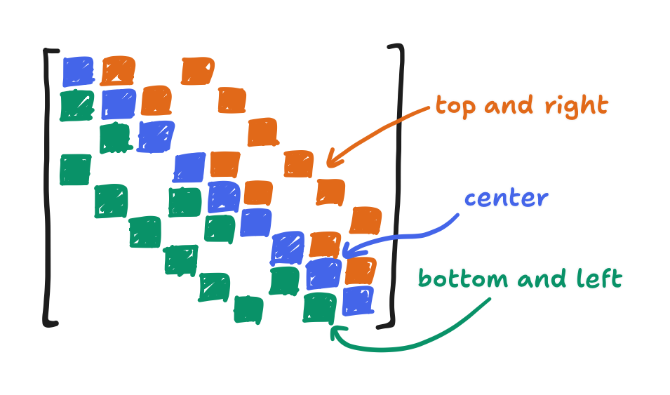
That aside, in this decomposition, it happens that $D$ is a diagonal matrix. As a result, we can say that its inverse $D^{-1}$ is just a matrix with reciprocals along the diagonal.
\[D^{-1} = \begin{bmatrix} a_{11}^{-1} \\ & a_{22}^{-1} \\ & & \ddots \\ & & & a_{nn}^{-1} \end{bmatrix}\]With that in mind, we can derive the following equation from $Ax = b$,
\[\begin{align*} A x & = b \\ (D + L + U) x & = b \\ Dx + (L+U)x & = b \\ Dx & = b - (L+U) x \\ x & = D^{-1} (b - (L+U) x) \end{align*}\]where $x$ appears in two places. From there, Jacobi iteration is to let the right-hand $x$ be some guess at the solution that we’ll call $x^{(k)}$ and let the left-hand $x$ be the updated guess $x^{(k+1)}$.
\[x^{(k+1)} = D^{-1} (b - (L+U) x^{(k)})\]In a moment, we’ll show that—given a specific condition holds—$x^{(k+1)}$ is always a better guess than $x^{(k)}$.
First, let’s see how the expression $D^{-1} (b - (L+U)x)$ manifests in practice. How is it faster than inverting $A$? Where do the sparse matrices come in? We just need to go get one element of $x^{(k+1)}$ at a time.
We know that $D^{-1}$, like $D$, is diagonal, and multiplying a vector by a diagonal matrix happens to be equivalent to multiplying each element with a corresponding $a_{ii}^{-1}$.
\[\begin{bmatrix} a_{11}^{-1} \\ & a_{22}^{-1} \\ & & \ddots \\ & & & a_{nn}^{-1} \end{bmatrix} \begin{bmatrix} x_1 \\ x_2 \\ \vdots \\ x_n \end{bmatrix} = \begin{bmatrix} a_{11}^{-1} x_1 \\ a_{22}^{-1} x_2 \\ \vdots \\ a_{nn}^{-1} x_n \end{bmatrix}\]So, to acquire some element of $x^{(k+1)}$, we can at least compute $b - (L+U) x^{(k)}$ in its entirety, pick the $i$-th element of that, then multiply it by $a_{ii}^{-1}$. Next, to subtract $(L+U)x^{(k)}$ from $b$ is of course equivalent to subtracting each element of $(L+U)x^{(k)}$ from the corresponding element of $b$. That leaves $(L+U)x^{(k)}$ by itself.
Well, remember where we came from: $A$ is a sparse because each of its rows is just an instance of the discretized Poisson’s equation centered at some point. Said equation only involves the center point and its neighbors. If $D$ contained all the center coefficients, then $L+U$ is just the neighbor coefficients. That is, the $i$-th element of $(L+U)x^{(k)}$ is just a sum of the four neighbor terms.
\[\frac{p[i+1, j] + p[i-1, j] + p[i, j+1] + p[i, j-1]}{\Delta x^2}\]It’s a sum of the four neighbor terms when there are four of them, anyway. So that I may keep it concise, whenever you see a $-4$ and four terms, please adjust it to a $-3$ and three terms or $-2$ and two terms at the boundary.
From the bottom to the top, $D^{-1}(b-(L+U)x^{(k)})$ can be computed one element at a time. It’s a composition of three operations: multiplication by $a_{ii}^{-1}$, subtraction from $b_i$, and the summing of the neighbor terms. If we put it all together, we get this:
\[p^{(k+1)}[i, j] = - \frac{\Delta x^2}{4} \left( d[i, j] - \frac{p^{(k)}[i+1, j] + p^{(k)}[i-1, j] + p^{(k)}[i, j+1] + p^{(k)}[i, j-1]}{\Delta x^2} \right)\]Apart from a bit of algebra, this is identical to the derivations of Jacobi iteration in Wong’s post and the GPU Gems article. Not bad!
Now, why is this fast? Instead of doing a matrix multiply the normal way, we’re just calculating an iteration rule on each element. If $A$ was not sparse, then a row of $(L+U)$ wouldn’t contain the four neighbors but rather roughly $N$ terms, and the complexity of one iteration would be $O(N^2)$. Instead, one iteration is $O(N)$! That’s far better than $O(N^3)$. The catch: if we iterate as many times it’ll take to achieve a fixed amount of improvement, the total complexity is higher, but I’ll consider that out-of-scope for today. We’ll instead iterate a fixed number of times and call it day. Here’s what the code for that would look like. Please forgive my extensive use of pointers here.
struct pois_context {
    float *d;
    float dx;
};

static inline int index(int i, int j, int dim_x) {
    return dim_x*j+i;
}

static float pois_expr_safe(float *p, int i, int j, int dim_x, int dim_y,
        void *ctx)
{
    struct pois_context *pois_ctx = (struct pois_context*)ctx;
    int i_max = dim_x-1, j_max = dim_y-1;

    float p_sum = 0;
    int a_ii = 0;
    if (i > 0) {
        p_sum += *(p-1);
        ++a_ii;
    }
    if (i < i_max) {
        p_sum += *(p+1);
        ++a_ii;
    }
    if (j > 0) {
        p_sum += *(p-dim_x);
        ++a_ii;
    }
    if (j < j_max) {
        p_sum += *(p+dim_x);
        ++a_ii;
    }

    static const float neg_a_ii_inv[5] = {0, 0, -1.0/2.0, -1.0/3.0, -1.0/4.0};
    int ij = index(i, j, dim_x);

    return neg_a_ii_inv[a_ii] * (pois_ctx->dx * pois_ctx->d[ij] - p_sum);
}

void poisson_solve(float *p, float *div, int dim_x, int dim_y, float dx,
        int iters, float *scratch)
{
    float *wrt = p, *rd = scratch, *temp;
    int ij;

    for (ij = 0; ij < dim_x*dim_y; ij++) {
        p[ij] = 0;
        scratch[ij] = 0;
    }

    struct pois_context pois_ctx = {.d = div, .dims = dims, .dx = dx};

    for (int k = 0; k < iters; k++) {
        for (int j = 0; j < dim_y; j++) {
            for (int i = 0; i < dim_x; i++) {
                ij = index(i, j, dim_x);
                wrt[ij] = pois_expr_safe(&rd[ij], i, j, dim_x, dim_y, &pois_ctx);
            }
        }
        temp = wrt;
        wrt = rd;
        rd = temp;
    }

    if (wrt == scratch) {
        for (ij = 0; ij < dim_x*dim_y; ij++) {
            p[ij] = scratch[ij];
        }
    }
}
However! If we want to run this on an ESP32, that is too many if statements to be going through in the main loop. Instead, if we sweep through all of the non-boundary elements first, we can skip those if statements. This creates a fast path.
Here’s what that looks like, on top of the previous code.
void domain_iter(float (*expr_safe)(float*, int, int, int, int, void*),
        float (*expr_fast)(float*, int, int, int, int, void*), U *wrt,
        T *rd, int dim_x, int dim_y, void *ctx)
{
    int i_max = (dim_x)-1, j_max = (dim_y)-1;  // inclusive!
    int ij, ij_alt;

    // Loop over the main body
    for (int j = 1; j < j_max; ++j) {
        for (int i = 1; i < i_max; ++i) {
            ij = index(i, j, dim_x);
            wrt[ij] = expr_fast(&rd[ij], i, j, dim_x, dim_y, ctx);
        }
    }

    // Loop over the top and bottom boundaries (including corners)
    for (int i = 0; i <= i_max; ++i) {
        ij = index(i, 0, dim_x);
        wrt[ij] = expr_safe(&rd[ij], i, 0, dim_x, dim_y, ctx);
        ij_alt = index(i, j_max, dim_x);
        wrt[ij_alt] = expr_safe(&rd[ij_alt], i, j_max, dim_x, dim_y, ctx);
    }

    // Loop over the left and right boundaries
    for (int j = 1; j < j_max; ++j) {
        ij = index(0, j, dim_x);
        wrt[ij] = expr_safe(&rd[ij], 0, j, dim_x, dim_y, ctx);
        ij_alt = index(i_max, j, dim_x);
        wrt[ij_alt] = expr_safe(&rd[ij_alt], i_max, j, dim_x, dim_y, ctx);
    }
}

static float pois_expr_fast(float *p, int i, int j, int dim_x, int dim_y,
        void *ctx)
{
    struct pois_context *pois_ctx = (struct pois_context*)ctx;

    float p_sum = ((*(p-1) + *(p+1)) + (*(p-dim_x) + *(p+dim_x)));

    int ij = index(i, j, dim_x);
    return -0.25f * (pois_ctx->dx * pois_ctx->d[ij] - p_sum);
}

void poisson_solve(float *p, float *div, int dim_x, int dim_y, float dx,
        int iters, float *scratch)
{
    float *wrt = p, *rd = scratch, *temp;

    for (int ij = 0; ij < dim_x*dim_y; ij++) {
        p[ij] = 0;
        scratch[ij] = 0;
    }

    struct pois_context pois_ctx = {.d = div, .dims = dims, .dx = dx};

    for (int k = 0; k < iters; k++) {
        domain_iter(pois_expr_safe, pois_expr_fast, wrt, rd, dim_x, dim_y,
            &pois_ctx);
        temp = wrt;
        wrt = rd;
        rd = temp;
    }

    if (wrt == scratch) {
        for (int ij = 0; ij < dim_x*dim_y; ij++) {
            p[ij] = scratch[ij];
        }
    }
}
That out of the way, why does the Jacobi method work in the first place?
Take the iteration rule and subtract the equation it comes from. Then, it reduces because the $b$ from both cancel.
\[\begin{align*} & & x^{(k+1)} & = D^{-1} (\cancel{b} - (L+U) x^{(k)} )\\ & -( & x & = D^{-1} (\cancel{b} - (L+U) x) & ) \\ \hline \\[-1em] & & x^{(k+1)} - x & = - D^{-1} (L+U) (x^{(k)} - x) \end{align*}\]Consider what $x^{(k+1)}-x$ and $x^{(k)}-x$ mean. They’re the error of our guesses! With every iteration, this error is multiplied by $-D^{-1} (L+U)$! Let’s call this matrix $C_\text{Jac}$.
For ease of explanation, let’s assume that $C_\text{Jac}$ can be diagonalized (for the otherwise defective matrices, there’s another way to go about this that’s similar). Because it can be diagonalized, the error can be expressed as a linear combination of its eigenvectors,
\[x^{(k)} - x = c_1^{(k)} v_1 + c_2^{(k)} v_2 + \dots + c_n^{(k)} v_n\]whereby each component gets multiplied by the corresponding eigenvalue in each iteration.
\[\begin{align*} x^{(k+1)} - x & = C_\text{Jac} (c_1^{(k)} v_1 + c_2^{(k)} v_2 + \dots + c_n^{(k)} v_n) \\ & = c_1^{(k)} C_\text{Jac} v_1 + c_2^{(k)} C_\text{Jac} v_2 + \dots + c_n^{(k)} C_\text{Jac} v_n \\ & = c_1^{(k)} \lambda_1 v_1 + c_2^{(k)} \lambda_2 v_2 + \dots + c_n^{(k)} \lambda_n v_n \end{align*}\]Let’s focus on a single term here—say $c_1^{(k)} \lambda_1 v_1$. On the next iteration, it gets multiplied by $C_\text{Jac}$ again, meaning that it becomes $c_1^{(k)} \lambda_1^2 v_1$. You can see that doing this repeatedly gets us an exponential series. The same can be said for the other terms. If any of the eigenvalues have a magnitude that is greater than one, then Jacobi iteration wouldn’t work because the error would explode. However, if all of the eigenvalues have magnitudes that are less than one, then the error would converge to zero. Hence the point: $x^{(k+1)}$ would always be a better guess than $x^{(k)}$.
The largest magnitude of all the eigenvalues is said to be the “spectral radius” of the matrix. Some of the eigenvalues having a magnitude over one is the same as the spectral radius being over one. All of them having a magnitude under one is the same as the spectral radius being under one. In the latter case, the eigenvector with the largest magnitude is decaying the slowest, but another way of looking at it is that all error decays at least as fast. For example, if the spectral radius of $C_\text{Jac}$ i.e. “$\rho(C_\text{Jac})$” is 0.9, then 20 iterations should cut the error by at least 88 percent. All-in-all, so long as the spectral radius is under one, Jacobi iteration can be used to solve our boundary value problem, giving the pressure field that appropriately fits the Helmholtz-Hodge decomposition.
That said, how can we know that it is? What is our spectral radius, actually? Well, about that…
I don’t know any proofs of one way or the other, but I just did provide a general—though not analytic—description of $A$. If we take some specific case of $A$, then there are iterative, sparse algorithms for (approximately) finding the eigenvalues and eigenvectors. In Python, the SciPy package offers one, scipy.sparse.linalg.eigs. Many months back, I thought that it would be perfect for finding the spectral radius. I wrote a script, and here it is.
import numpy as np
from math import prod
from matplotlib import pyplot as plt
import scipy.linalg
from scipy.sparse import csr_array, eye
import scipy.sparse.linalg

DX = 1.0
N_EIGS = 20
N_ROWS = 60
N_COLS = 80


def plot_eigs(
    arr: csr_array, subplots: tuple[int, int], neg_first: bool = True, digits: int = 5
):
    n_eigs = prod(subplots)

    eigs, v = scipy.sparse.linalg.eigs(arr, k=n_eigs, which="LM")

    # I haven't seen non-real values, so don't show them for legibility
    if np.any(np.imag(eigs)) or np.any(np.imag(v)):
        print("warning: eigenvalues or eigenvectors have an imaginary component")
    eigs = np.real(eigs)
    v = np.real(v)

    # round the eigenvalues for legibility, but check for ambiguity
    eigs = np.round(eigs, digits)
    pairwise_matches = np.count_nonzero(
        eigs[:, np.newaxis] == eigs[np.newaxis, :], axis=1
    )
    if np.any((pairwise_matches > 1) & (eigs != 0)):  # ignore self-match and zero
        print("warning: rounding has made some eigenvalues ambiguous")

    # in case of a pos-neg pair, strictly show pos or neg first
    is_pos = eigs > 0
    if neg_first:  # pos first, then the stable descending sort flips that
        eigs = np.hstack([eigs[is_pos], eigs[~is_pos]])
        v = np.hstack([v[:, is_pos], v[:, ~is_pos]])
    else:  # neg first, then the stable descending sort flips that
        eigs = np.hstack([eigs[~is_pos], eigs[is_pos]])
        v = np.hstack([v[:, ~is_pos], v[:, is_pos]])
    permute = np.argsort(np.abs(eigs), stable=True)[::-1]
    eigs = eigs[permute]
    v = v[:, permute]

    MIN_RANGE = 1e-9
    for i in range(n_eigs):
        eigenvector = v[:, i].reshape((N_ROWS, N_COLS))
        v_min = np.min(eigenvector)
        v_max = np.max(eigenvector)
        if v_max - v_min < MIN_RANGE:  # probably a flat plane
            v_max += MIN_RANGE
            v_min -= MIN_RANGE
        plt.subplot(*subplots, i+1)
        plt.imshow(eigenvector, vmin=v_min, vmax=v_max, cmap="coolwarm")
        plt.axis("off")
        plt.title('$\\lambda$ = %0.*f' % (digits, eigs[i]))

    plt.tight_layout()


op = scipy.sparse.linalg.LaplacianNd((N_ROWS, N_COLS), boundary_conditions="neumann")
arr = (1 / (DX ** 2)) * csr_array(op.tosparse(), dtype=np.float64)

# Jacobi
diag_inv = arr.diagonal(0) ** -1
lu = arr.copy()
lu.setdiag(0, 0)
iter_matrix_jacobi = diag_inv[:, np.newaxis] * lu  # implements D^(-1) (L + U)
plot_eigs(iter_matrix_jacobi, (3, 4), neg_first=True)
plt.savefig("eigs_jacobi.png", dpi=300)
plt.cla()

# Richardson
omega = (DX ** 2) / -4
iter_matrix_richardson = csr_array(eye(arr.shape[0]), dtype=np.float64) - omega * arr
plot_eigs(iter_matrix_richardson, (3, 4), False)
plt.savefig("eigs_richardson.png", dpi=300)
plt.cla()
Given some $\Delta x$ and some grid, it calculates $A$, calculates $C_\text{Jac}$ from $A$ (and $C_\text{Richardson}$, but we’ll get to that) then finds the top twenty eigenvalues with the largest magnitude—plus the corresponding eigenvectors. Then, the spectral radius is just taking the first largest magnitude. It’s not useful for making a general statement about all cases of $A$, but it’s all I need for my specific case. I also went ahead here and reshaped the eigenvectors back into arrays, letting us visualize whatever eigenvector getting hit with so-and-so eigenvalue as the component of a field getting diminished.
In the case of ESP32-fluid-simulation, I was limited by the ESP32’s RAM to a $60 \times 80$ grid, and I happened to let $\Delta x = 1$. Given that, the script got this:
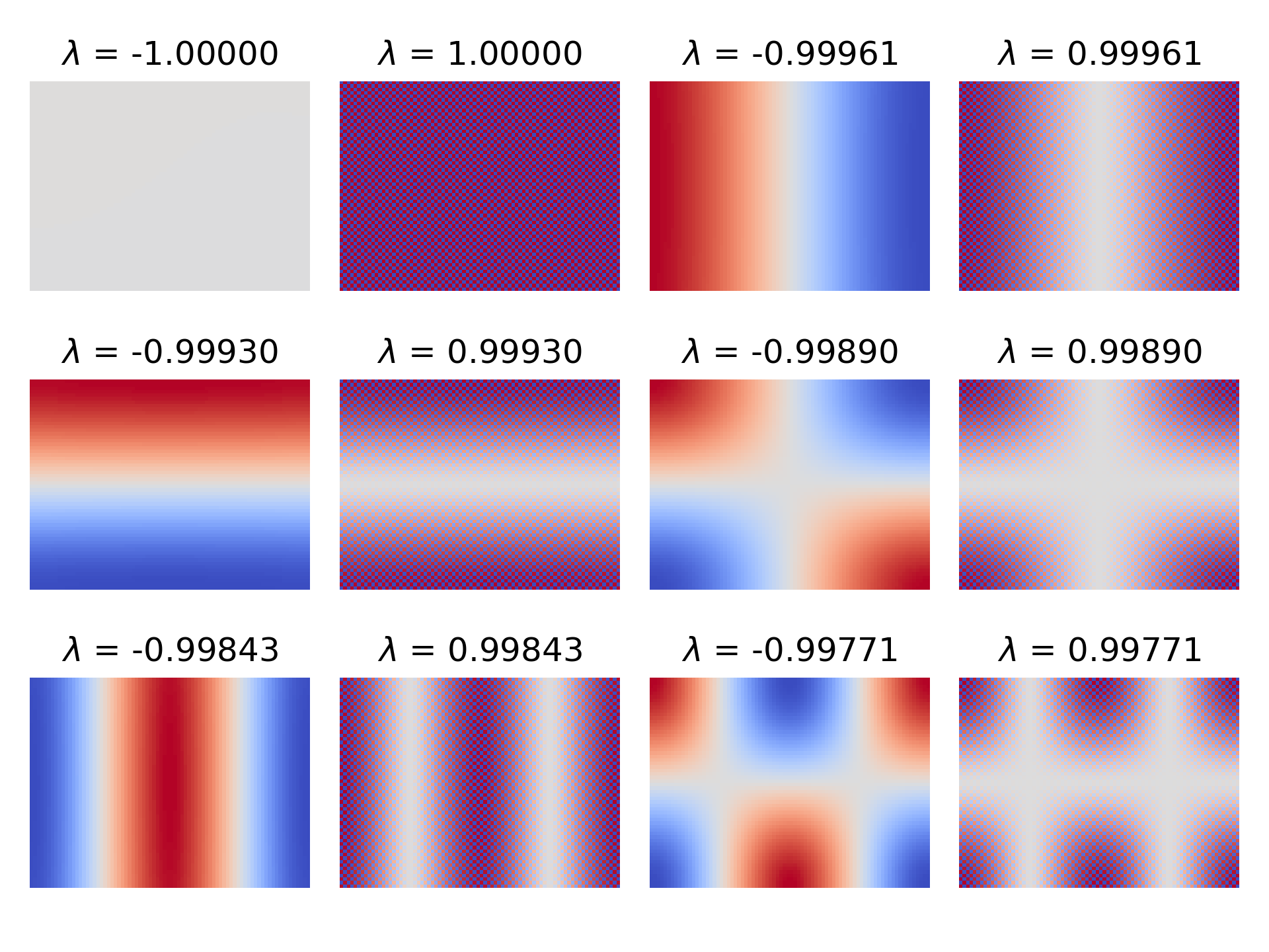
Immediately, we can notice two things:
1) The spectral radius of $C_\text{Jac}$ appears to be not less than one because two of the eigenvalues are $1$ and $-1$.
2) There seems to be positive-negative pairs of eigenvalues, with the eigenvector associated with the positive one looking like the negative counterpart but multiplied by a checkerboard pattern.
From what I’ve gathered, both of these things are to be expected.
Regarding (2), following linked references on Wikipedia led me to a 1950 PhD thesis by David M. Young—an analysis of “successive over-relaxation” in the context of finite difference schemes. Setting aside what “successive over-relaxation” is for now, I worked out that $A$ happens to satisfy what Young calls “property A”. In fact, Young was deriving results from this “property A” with a finite difference problem like this in mind! The thesis is publicly available if you want to see how Young describes it exactly, but in this context, it’s this: given $A$ only has points interact with their neighbors, the grid can be divided into a succession of sets of points where each set only interacts with the preceding and the succeeding set.
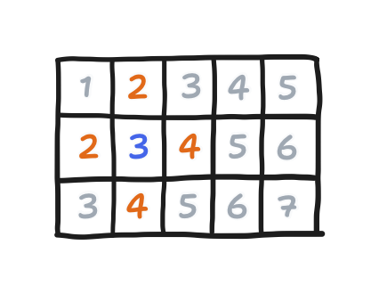
Because property A is satisfied, much of the conclusions of that analysis follow. That includes a theorem that the eigenvalues of Jacobi iteration (which he called the “Kormes method”, apparently) will come in positive-negative pairs, associated with a pair of eigenvectors where one is just a copy of the other but multiplied by $1$ and $-1$ alternating. That’s exactly what we’re seeing here!
As you might expect, we’ll be interested in Property A and “successive over-relaxation” soon.
Regarding (1), I found a StackExchange post that states that an $A$ constructed from a boundary value problem with only i.e. “purely” Neumann boundaries must have infinitely many solutions, separated by a constant, because the entire boundary value problem, which is just the governing equations (which are partial differential equations) and the boundary conditions, then only concerns the derivative of the pressure field. It’s like tacking on “$+\;C$” to the end of an indefinite integral’s result. That means there needs to be a place to choose that constant.
Looking at the eigenvector corresponding to $-1$: it’s very flat. As a flat component that doesn’t diminish over iterations, it looks to me like setting the initial weight of this component is equivalent to choosing the constant part of the solution.
In my case, I always started with a zeroed-out field as the first guess, which zeroes out that component too. But in any case, the neat part is that the choice of constant doesn’t matter because we ultimately subtract the gradient of the pressure from the uncorrected velocity. The gradient consists of partial derivatives, and the constant part doesn’t change its value. The same can be said for its checkerboard counterpart because the discrete gradient always happens to use points with the same color, so to speak. In other words, we’re free to take the next largest eigenvalue as our “spectral radius”—to abuse the term a bit. For our $60 \times 80$ grid and $\Delta x = 1$, that’s $0.9996$. We can be sure that Jacobi iteration solves the boundary value problem.
One more “but actually” before we move on: I mentioned that my script can also calculate $C_\text{Richardson}$. I noticed in my sources that their codes for computing Jacobi iteration element-wise didn’t exactly do $D^{-1} (b - (L+U) x^{(k)})$. When it came time to multiply by $a_{ii}^{-1}$, which can be either $-\frac{\Delta x^2}{4}$, $-\frac{\Delta x^2}{3}$, or $-\frac{\Delta x^2}{2}$ depending on whether the $i$-th point is at the boundary, they strictly multiplied by $-\frac{\Delta x^2}{4}$ instead. At the same time, instead of making sure to not take the top neighbor at the top boundary, left neighbor at the left boundary, et cetera, and they pulled the ghost row/column value instead. I realized later that this was technically Richardson iteration.
Richardson iteration comes from a different splitting of $A$ into a diagonal matrix of constants and the remainder.
\[A = \alpha I + (A - \alpha I)\]With this sum, we can do the following derivation from $Ax = b$, like we did for Jacobi iteration.
\[\begin{align*} Ax & = b \\ (\alpha I + (A - \alpha I)) x & = b \\ \alpha I x + (A - \alpha I) x & = b \\ \alpha I x & = b - (A - \alpha I) x \\ x & = \alpha^{-1} I (b - (A - \alpha I)x) \\ & = \alpha^{-1} b - \alpha^{-1} (A - \alpha I) x \\ & = \alpha^{-1} b + (I - \alpha^{-1} A) x \\ & \left\downarrow \text{Let }\omega = \alpha^{-1} \right. \\ & = \omega b + (I - \omega A) x\end{align*}\]We can also turn that into the following iteration rule.
\[x^{(k+1)} = \omega b + (I - \omega A) x^{(k)}\]Consider letting $\alpha = \frac{-4}{\Delta x^2}$ (conversely $\omega = \frac{\Delta x^2}{-4}$) so that $\alpha$ is exactly $a_{ii}$ if all four neighbors were there. Then, if $\alpha I$ is subtracted from $A$, a zero remains where $a_{ii}$ once was. Now, notice in the derivation how $(A - \alpha I)$ times $-\alpha^{-1}$ is $I - \omega A$. If there was a zero on the diagonal of $(A - \alpha I)$, there’s still a zero there in $I - \omega A$. This says the pressure at the center isn’t in play, like how it’s not in Jacobi iteration. Overall, it can be shown that Richardson iteration and Jacobi iteration happen to be identical in our problem, except at the boundary.
There, $a_{ii}$ is $\frac{-3}{\Delta x^2}$ or $\frac{-2}{\Delta x^2}$, and $-\frac{1}{4}$ or $-\frac{2}{4}$ is left, not zero, and then the pressure at the center point gets pulled in. When this is compared to how Stam’s “Real-Time Fluid Dynamics for Games” and the GPU Gems article pull a value from the ghost row/column, which in turn pulls from the center, it can be shown that what they’re doing is actually Richardson iteration! (Stam doesn’t do Richardson iteration to the tee, but we’ll get to that.)
When it comes to code, those articles proceed to use the ghost rows and columns as actual rows and columns in memory that are kept up-to-date. That lets them use the fast path on every point because every point does then have all four neighbors. This also has the same function run on all points, which is important for GPUs. But for us, that idea is incompatible with the C code I’ve shown so far. At the very least, Richardson iteration could still be achieved by updating the safe path code, and we wouldn’t need to update the fast path code because that part is the same.
static float pois_expr_safe(float *p, int i, int j, int dim_x, int dim_y,
        void *ctx)
{
    struct pois_context *pois_ctx = (struct pois_context*)ctx;
    int i_max = dim_x-1, j_max = dim_y-1;

    float p_sum = 0;
    p_sum += (i > 0) ? *(p-1) : *p;
    p_sum += (i < i_max) ? *(p+1) : *p;
    p_sum += (j > 0) ? *(p-dim_x) : *p;
    p_sum += (j < j_max) ? *(p+dim_x) : *p;

    int ij = INDEX(i, j, dim_x);
    return -0.25 * (pois_ctx->dx * pois_ctx->d[ij] - p_sum);
}
That’s besides the point I wanted to make, though. Since they actually used Richardson iteration, I wanted to make sure that the spectral radius of $C_\text{Richardson}$ was also under one, so I added on to the script. To do that, I just needed to know what matrix the error gets multiplied by, and we can use the same equation subtraction as before to find that it’s $(I - \omega A)$.
\[\begin{align*} & & x^{(k+1)} & = \cancel{\omega b} + (I - \omega A) x^{(k)}\\ & -( & x & = \cancel{\omega b} + (I - \omega A) x & ) \\ \hline \\[-1em] & & x^{(k+1)} - x & = (I - \omega A) (x^{(k)} - x) \end{align*}\]Here’s its eigenvalues and eigenvectors for the $60 \times 80$ grid and $\Delta x = 1$:
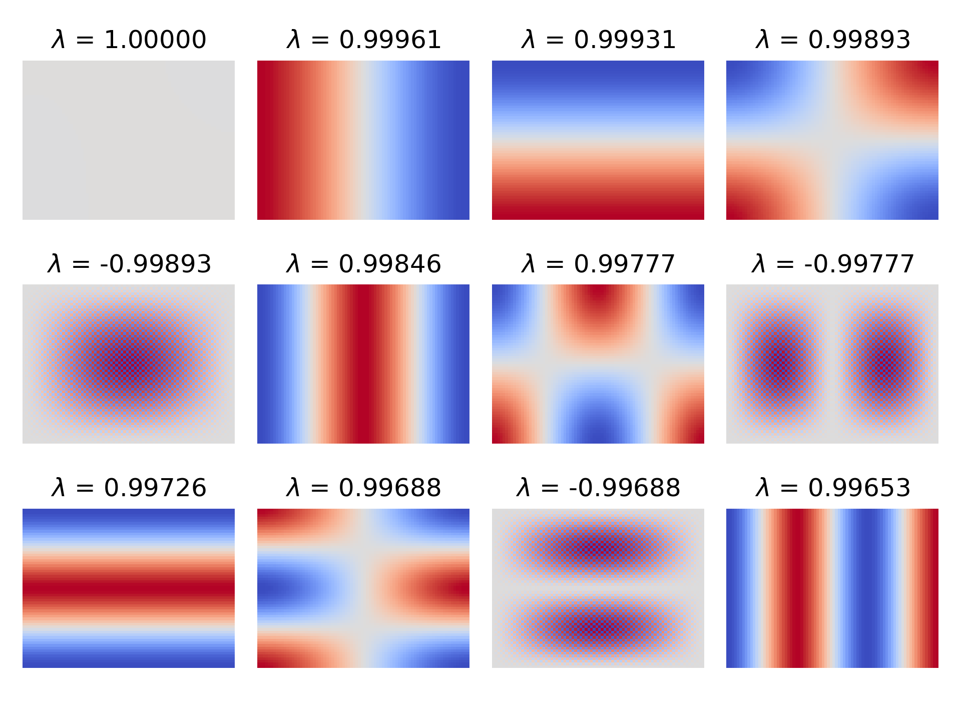
Though the eigenvectors are somewhat different, the spectral radius is close to that of Jacobi iteration—completely within rounding error in this case. It makes sense, given that $-\frac{4}{\Delta x^2}$ was the typical value on the diagonal. So, I wouldn’t be so concerned with the distinction, but I know I should at least point it out.
By showing exactly how Jacobi iteration manifests into code via sparse matrices and discussing the spectral radius, we’ve covered all the context that I once used to go beyond. Let’s start with a motivating question: why did I need to go beyond in the first place? The answer lies in the spectral radius we just found. With a spectral radius of $0.9996$, how many iterations would it take to cut the error by 90 percent? 5755 iterations! We can never hope to just use Jacobi iteration on an ESP32.
The first step beyond is to use “Gauss-Seidel” iteration instead. We’ll get to how to derive it, but I think it’s better to start with an interesting motivator. Classical “Gauss-Seidel” iteration is eerily similar to Jacobi iteration in implementation. Instead of element-wise assembling the next pressure array in an output memory, what if we compute it in the same memory as the current pressure array—overwriting one element at a time? Here’s what that would look like.
void poisson_solve(float *p, float *div, int dim_x, int dim_y, float dx,
        int iters, float omega)
{
    for (int ij = 0; ij < dim_x*dim_y; ij++) {
        p[ij] = 0;
    }
    struct pois_context pois_ctx = {.d = div, .dx = dx};
    for (int k = 0; k < iters; k++) {
        domain_iter(pois_expr_safe, pois_expr_fast, p, p, dim_x, dim_y,
            &pois_ctx);
    }
}
Simpler, no? It sounds like taking a shortcut at the cost of correctness, but this happens to give us the classical case of “Gauss-Seidel”. By doing this, we happen to use the values of the next pressure array when we pull the bottom and left neighbors, and we can converge faster for doing so. That’s the quintessential part of it. Naturally, Stam’s method of choice in “Real-Time Fluid Dynamics for Games” was Gauss-Seidel, or—to be precise—a Gauss-Seidel-ized Richardson iteration. I don’t think the difference matters much. Meanwhile, the GPU Gems article sticks with doing many Jacobi iterations, probably because immediately using elements that were just calculated makes GPU parallelization awkward.
What does matter is this: in Jacobi iteration, we could have looped through the elements in any order with no impact, but in Gauss-Seidel iteration, the order does have an impact. The code we just saw happens to loop through the elements in the conventional left-to-right bottom-to-top order, and doing so pulls the from the bottom and left immediately. That’s the “classical” case, but there’s also “red-black Gauss-Seidel iteration”. Its only difference is in the order.
Imagine the grid being colored in a checkerboard red-black pattern, where black points only neighbor red points and red points only neighbor black points. “Red-black” iteration is to just visit all of the red points then to visit all of the black points only after (or all black points then red points). Anyway, the result is this: in the first half, none of the neighbors are of the next pressure array, but in the second half, all of them are.
\[p^{(k+1)}[i, j] = \begin{cases} \displaystyle - \frac{\Delta x}{4} \left( d[i, j] - \frac{p^{(k)}[i+1, j] + p^{(k)}[i-1, j] + p^{(k)}[i, j+1] + p^{(k)}[i, j-1]}{\Delta x^{2}} \right) & \text{red } i, j \\[1em] \displaystyle - \frac{\Delta x}{4} \left( d[i, j] - \frac{p^{(k+1)}[i+1, j] + p^{(k+1)}[i-1, j] + p^{(k+1)}[i, j+1] + p^{(k+1)}[i, j-1]}{\Delta x^{2}} \right) & \text{black } i, j \end{cases}\]For thinking about what the code for such a peculiar looping would be, here are the two key tricks:
-
all points one step (horizontal or vertical) away are the other color,
-
all points two steps away are the same color, and
-
if we assume that point $0,\;0$ is black, then every point where $i+j$ is even must be black.
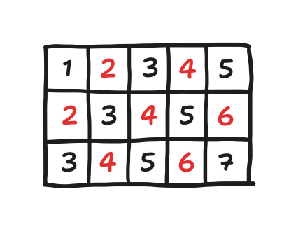
And now, here’s what the code for that would look like.
static inline int point_is_red(int i, int j) {
    return (i + j) & 0x1;
}

static void domain_iter_red_black(
    float (*expr_safe)(float*, int, int, int, int, void*),
    float (*expr_fast)(float*, int, int, int, int, void*), U *wrt, T *rd,
    int dim_x, int dim_y, void *ctx)
{
    int i_max = (dim_x)-1, j_max = (dim_y)-1;  // inclusive!
    int ij, offset;

    int bottom_left_is_red = point_is_red(0, 0),
        bottom_right_is_red = point_is_red(i_max, 0),
        top_left_is_red = point_is_red(0, j_max);

    int on_red = 0;
    repeat_on_red:  // on arrival to this label, on_red = 1

    // Loop over the main body (starting from 1,1 as black or 2,1 as red)
    for (int j = 1, offset = on_red; j < j_max; ++j, offset ^= 1) {
        for (int i = 1+offset; i < i_max; i += 2) {
            ij = index(i, j, dim_x);
            wrt[ij] = expr_fast(&rd[ij], i, j, dim_x, dim_y, ctx);
        }
    }

    // Loop over the bottom (including left and right corners)
    offset = (on_red == bottom_left_is_red) ? 0 : 1;
    for(int i = offset; i <= i_max; i += 2) {
        ij = index(i, 0, dim_x);
        wrt[ij] = expr_safe(&rd[ij], i, 0, dim_x, dim_y, ctx);
    }

    // Loop over the top (including left and right corners)
    offset = (on_red == top_left_is_red)? 0 : 1;
    for(int i = offset; i <= i_max; i += 2) {
        ij = index(i, j_max, dim_x);
        wrt[ij] = expr_safe(&rd[ij], i, j_max, dim_x, dim_y, ctx);
    }

    // Loop over the left (starting from 0,1 or 0,2)
    offset = (on_red == !bottom_left_is_red) ? 1 : 2;  // we're *adjacent* it
    for(int j = offset; j < j_max; j += 2) {
        ij = index(0, j, dim_x);
        wrt[ij] = expr_safe(&rd[ij], 0, j, dim_x, dim_y, ctx);
    }

    // Loop over the right (starting from i_max,1 or i_max,2)
    offset = (on_red == !bottom_right_is_red)? 1 : 2;
    for(int j = offset; j < j_max; j += 2) {
        ij = index(i_max, j, dim_x);
        wrt[ij] = expr_safe(&rd[ij], i_max, j, dim_x, dim_y, ctx);
    }

    if (!on_red) {
        on_red = 1;
        goto repeat_on_red;
    }
}
The change in going with this over classical Gauss-Seidel isn’t critical. I just did it because it made the sim look better. Though to be frank, I’m not sure why. In fact, by starting from what’s presented in Young’s analysis, it can be shown that both methods have the same spectral radius. I’ll get to that at some point.
I think Gauss-Seidel iteration is better thought of as an improvement that emerges from taking the shortcut in the element-wise computation, but if you’re curious, here’s how it emerges when starting from the linear algebra. Recall the $A = D + L + U$ splitting, and let $S$ be the diagonal plus the lower-triangular parts, $D + L$. Like in Jacobi iteration and Richardson iteration, we derive something from $Ax = b$.
\[\begin{align*} Ax & = b \\ (S+U) x & = b \\ Sx + Ux & = b \\ x & = S^{-1} (b - Ux)\end{align*}\]However, we now have to do something slightly different when we’re going element by element. Calculating $b - Ux$ is the same, but how on earth do we compute the multiplication of $b - Ux$ with $S^{-1}$? We exploit the fact that $S$ is sparse and lower-triangular. (If you’re confused, “lower-triangular” can include a non-zero diagonal, whereas a “strictly lower-triangular” one cannot.)
There’s two issues at hand here: (1) we need to compute individual elements of $S^{-1} (b - Ux)$, and (2) we don’t even know what $S^{-1}$ is. Dealing with the likewise issues of $D$ in Jacobi iteration and $\alpha I$ in Richardson iteration was easier because those were diagonal matrices. Fortunately, $S$ being lower-triangular lets us kill two birds with one stone by using forward substitution.
Forward substitution is analogous to the latter half of Gaussian elimination. First, recognize that calculating the multiplication $S^{-1} (b - Ux)$ is equivalent to solving the equation $Sz = (b-Ux)$ for $z$. Solving this equation sidesteps needing to know $S^{-1}$, and forward substitution happens to solve for $z$ one element at a time. To show it, let’s first recast problem into another $Ax = b$, where $A$ is $S$, $b$ is $(b-Ux)$, and $x$ is what we’re looking for. Then, we should write out each individual equation.
\[\begin{align*} & a_{11} x_1 & & = b_1 \\ & a_{21} x_1 + a_{22} x_2 & & = b_2 \\ & & & \enspace \vdots \\ & a_{n1} x_1 + a_{n2} x_2 + \dots + a_{nn} x_n & & = b_n \end{align*}\]The first equation is obvious, $x_1 = \frac{b_1}{a_{11}}$. Then, we can substitute $x_1$ into all the following equations. That makes the second equation solvable, yielding $x_2 = \frac{1}{a_{22}} (b_2 - a_{21} x_1)$. Substituting this result downward makes the third equation solvable, and so on. Yielding one element at a time, this solves $A x = b$, or in other words computes $A^{-1} b$.
Look at how forward substitution calculates one element at a time, and in particular how it pulls elements of $b$. The first equation uses $b_1$, the second uses $b_2$, and so on. So, can we not interleave the computation of elements of $x$ and $b$? We can calculate $b_1$ then $x_1$, $b_2$ then $x_2$, and so on. Now, remember that “$b$” here is $b - Ux$ and “$x$” here is $z$ i.e. $S^{-1} (b - Ux)$. Computing some element of “$b_i$” involves the right and top neighbors of point $i$ (since $U$ is upper-triangular), and computing “$x_i$” involves the substituted-in elements of $x$ from the bottom and left neighbors (since $S$ is lower-triangular). Et voila, we’ve arrived at the same classical Gauss-Seidel code!
Finally, the difference between this and red-black Gauss-Seidel is this: by looping through the red points then through the black points, we’ve permuted the elements of $x$ (from the original $Ax = b$) into a new order that follows this looping, an order distinct from the conventional left-to-right bottom-to-top mapping from 2D position to 1D index. That’s best demonstrated with our good old three-by-three example.
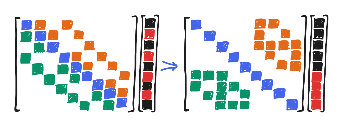
Feel free to notice here how all the red points and black points are consecutive now!
Formally, this can be written as a matrix similarity between $A$ and what we’ll call $A_\text{red-black}$, with a permutation matrix $P$ as the change-of-basis.
\[P^{-1} A_\text{red-black} P = A\]Then, $Ax = b$ can be written as $P^{-1} A_\text{red-black} P x = b$. This expresses how the elements of $x$ are permuted, put through $A_\text{red-black}$, then permuted back into conventional order. That said, the red-black code doesn’t actually shuffle the memory, and rather the changed looping does the work.
Last but not least, the next step beyond Gauss-Seidel iteration is “successive over-relaxation”, or “SOR”. The intuition of it goes like this: if stepping from $p^{(k)}[i, j]$ to $p^{(k+1)}[i, j]$ is in the right direction, what if we went further in that direction? It’s a linear extrapolation from $p^{(k)}[i, j]$ to $p^{(k+1)}[i, j]$ and onward. It quite literally is the same expression as linear interpolation (yes, that lerp). That is,
\[p_\text{SOR}^{(k+1)}[i, j] = \omega p_\text{G-S}^{(k+1)}[i, j] + (1-\omega) p^{(k)}[i, j]\]where $p_\text{G-S}^{(k+1)}[i, j]$ is the result from Gauss-Seidel iteration and $\omega$ is ordinarily a parameter between $0$ and $1$ that slides us between $p_\text{G-S}^{(k+1)}[i, j]$ and $p^{(k)}[i, j]$. But here, given some conditions are met, we’re free to push $\omega$ beyond $1$. Doing so can get us closer to the solution faster—much faster. Let’s finally get into what spectral radius we get.
So far, we have had nothing concrete to say about the spectral radius of Gauss-Seidel iteration—not what we can expect it to be, much less whether it is better than Jacobi iteration. The same can be said for SOR. To preface a bit first, you may have already realized that Gauss-Seidel can also be thought of as the $\omega = 1$ case of SOR. This means that an analysis of SOR will also cover Gauss-Seidel. That out of the way, Young found that, for matrices satisfying Property A, the spectral radius of SOR is a function of $\omega$ and the spectral radius of Jacobi iteration! Denoting $\rho(C_\text{Jac})$ as $\mu$ here, it goes like this:
\[\rho(C_\omega) = \begin{cases} \frac{1}{4} \left( \omega \mu + \sqrt{\omega^2\mu^2 - 4(\omega-1)} \right)^2 & 0 \leq \omega \leq \omega_\text{opt} \\ \omega - 1 & \omega_\text{opt} \leq \omega \leq 2 \end{cases}\]where $\omega_\text{opt}$ is the value of $\omega$ that minimizes $\rho(C_\omega)$ and is given by the following expression
\[1 + \left( \frac{\mu}{1+\sqrt{1-\mu^2}} \right)^2\]
With this, we can check out what the radius of Gauss-Seidel iteration is. Plugging $1$ into the formula, we get that
\[\begin{align*}\rho(C_1) & = \frac{1}{4} \left( \mu + \sqrt{\mu^2} \right)^2 \\ & = \frac{1}{4} (2\mu)^2 \\ & = \mu^2 \end{align*}\]meaning that one Gauss-Seidel step is worth two Jacobi steps.
Now, let’s see how many Jacobi steps one SOR step is worth. Given our $60 \times 80$ grid and $\Delta x = 1$, we found earlier that our spectral radius was $0.9996$. Letting $\mu = 0.9996$, we get that $\omega_\text{opt} = 1.96$. Passing this into the formula for $\rho(C_\omega)$, we get that $\rho(C_{1.96}) = 0.96$. The number of steps is the exponent that takes $0.9996$ to $0.96$, or in other words $\log_{0.9996}(0.96) = 102.034$. One step of SOR is worth over a hundred Jacobi steps. Granted, at this point, my sense for things being too good to be true leads me to suspect that we here have pushed the ideas of SOR to their breaking point. Here, I suspect that the “conjugate gradient” method makes more sense. In fact, in that response I got from Stam, he mentioned that it was what he used to find the pressure, along with using a MAC grid. Though the grids aren’t the same, it sounds like it could work, but that must be a side project for another day. This has been a long post, and this has been a long series.
This series has had more than a few tangents, and this one will be the last. I had seen the red-black order’s output looked much better than going in conventional order, so why did I assert that their spectral radii are the same?
First, actually, the order matters in Young’s derivation of SOR’s spectral radius. It only holds if the order is what he called a “consistent order”. After going through what makes a “consistent order”, he went on to show four cases. Red-black is in indeed one of them, but the conventional order is also one. To list them all, there is
- $\sigma_1$, a left-to-right, top-to-bottom order (equivalent to left-to-right, bottom-to-top),
- $\sigma_2$, a wavefront order,
- $\sigma_3$, the red-black order, and
- $\sigma_4$, a zigzag order.
You can see those orderings below. Points are in the order given by their numbers, though points with the same number can be evaluated in any order.
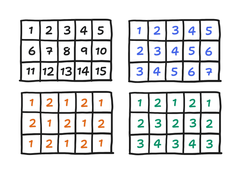
Because order doesn’t matter in Jacobi iteration, all orderings lead to the same $\rho(C_\text{Jacobi})$. Now, for a consistent order, $\rho(C_\omega)$ is a function of $\rho(C_\text{Jacobi})$. If the latter is the same, then so should be the former.
Yet they look different when I actually run the two. Perhaps they have different eigenvectors? I don’t know why that is, really, but I went ahead and picked red-black SOR because there was no arguing against the fact that it looked better.
Here’s the culminating piece, a red-black SOR code, the thing that made ESP32-fluid-simulation possible.
struct pois_context {
    float *d;
    float dx;
    float omega;
};

static float pois_sor_safe(float *p, int i, int j, int dim_x, int dim_y,
        void *ctx)
{
    struct pois_context *pois_ctx = (struct pois_context*)ctx;
    float omega = pois_ctx->omega;
    float p_gs = pois_expr_safe(p, i, j, dim_x, dim_y, ctx);
    return (1-omega)*(*p) + omega*p_gs;
}

static float pois_sor_fast(float *p, int i, int j, int dim_x, int dim_y,
        void *ctx)
{
    struct pois_context *pois_ctx = (struct pois_context*)ctx;
    float omega = pois_ctx->omega;

    float p_sum = (*(p-1) + *(p+1)) + (*(p-dim_x) + *(p+dim_x));

    int ij = index(i, j, dim_x);
    float p_gs = -0.25f * (pois_ctx->dx * pois_ctx->d[ij] - p_sum);

    return (1-omega)*(*p) + omega*p_gs;
}

void poisson_solve(float *p, float *div, int dim_x, int dim_y, float dx,
        int iters, float omega)
{
    for (int ij = 0; ij < dim_x*dim_y; ij++) {
        p[ij] = 0;
    }
    struct pois_context pois_ctx = {.d = div, .dx = dx, .omega = omega};
    for (int k = 0; k < iters; k++) {
        domain_iter_red_black(pois_sor_safe, pois_sor_fast, p, p, dim_x, dim_y,
            &pois_ctx);
    }
}
In summary, to compute a divergence-free velocity field, we applied the Helmholtz-Hodge decomposition, but the decomposition itself gave us a boundary value problem to solve. Through discretization, we turned that problem into a massive $Ax = b$ problem, but one where $A$ was sparse. We used that sparsity to our advantage, choosing to approximately solve it with an iterative method that lets us compute $x$ one step at a time and one element at a time—skipping the zeroes along the way. The first one we saw was Jacobi iteration. I shared how I got its spectral radius. Then, we saw Gauss-Seidel iteration and SOR. Finally, we learned that, for the class of matrices satisfying Property A, including our $A$, Gauss-Seidel was faster and SOR was dramatically faster. All this context was necessary to figuring out how to run a fluid sim on an ESP32.
With that, the actual fluid sim mechanism in ESP32-fluid-simulation is entirely covered, and that caps off the tour through its use of FreeRTOS, the Cheap Yellow Display (CYD), and the Navier-Stokes equations. This was quite the epic undertaking for me, building the sim more than one year ago then going to write on and off about it since. I’d do it again, considering that—in trying to explain it—I ended up formalizing my own understanding of my own project and updated it accordingly along the way. And now that understanding is here on the internet.
That said, this project is far from the last one I’ll ever make then write about. Look out for the next series, to be announced some day. In any case and for the last time, you can see ESP32-fluid-simulation on GitHub!