Detecting motion in RPLIDAR data using optical flow
Over a week, I happened to hack together an interesting procedure that ended up being an important part of the senior capstone project I was contributing to. The objective of this procedure: if it moves…
…detect it! The sensor involved here is the RPLIDAR, a low-cost “laser range scanner” that yields distances from itself at all angles. The principle behind the procedure is “optical flow”, a whole class of techniques for inferring the velocity of an object in a video by looking from frame to frame. The specific technique I used is a classic called the “Lucas-Kanade method”. It turned out that the same reasoning that constructs it (and optical flow more generally) also works with the data taken from the RPLIDAR.
That said, there has to be a fair bit of preprocessing on that data beforehand. I think the preprocessing itself poses an interesting introduction to some backgrounds though, so I’ll cover it too. To see this whole procedure, we’ll use the below example data to visualize the steps. Before, I used that data to devise the procedure in the first place, and it had been collected for me by someone else.
First, the RPLIDAR yields an irregular sampling of the room around it for a variety of reasons—from protocol overhead to measurement failure. Some may call this kind of data “unstructured”. On the other hand, with video essentially being a grid of dynamically updating pixels, optical flow expects regularly-sampled data. One easy-to-see solution to this is an “interpolation”. The general idea behind “interpolation” is to construct a continuous function that goes through discrete samples, unstructured or not, then collect new, regularly-sampled data from the function.
At the time, I chose to use “radial basis function” (RBF) interpolation. However, that ended up being a poor choice because something about the data forced me to accept a very relaxed form of it. What do I mean here? The result of an interpolation is not necessarily smooth. The simplest kind of interpolation, linear interpolation or “lerp”, is just connecting the samples with straight lines.
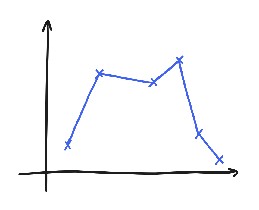
Linear interpolations can be extremely jagged for some data. RBF interpolation promises a degree of smoothness on the other hand, but it can also simply fail—to put it shortly. Explaining exactly how it fails seems a bit beyond the scope here, but suffice it to say that it failed here. The result of that failure was the relaxed form, and it amounted to a kind of curve-fitting. Though it still yielded a smooth, continuous function, it no longer went through the points. Well, curve-fitting is another solution to this problem, anyway. We can collect regularly-sampled data from it too.
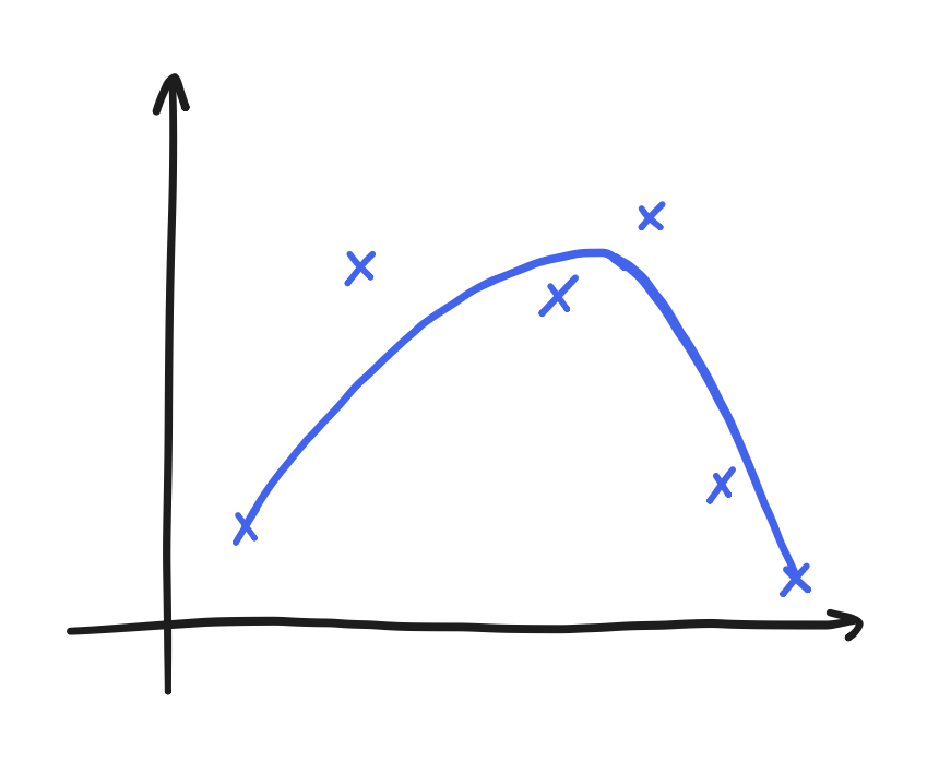
Here, let’s use a proper curve-fitting procedure in the first place! A good one is the Python make_smoothing_spline function offered by SciPy. This routine has some peculiarities, so I’ll leave here an Interpolator class that has a working use of it.
class Interpolator:
    def __init__(self, memory_size=512, lam=1e-3):
        self.memory = np.zeros((memory_size, 2))
        self.lam = lam

    def update(self, samples):
        self.memory = np.roll(self.memory, -len(samples), axis=0)
        self.memory[-len(samples):] = samples

    def take(self, x):
        # get samples in ascending order of angle
        angles = self.memory[:, 0]
        argsort_angles = np.argsort(angles)
        angles = angles[argsort_angles]
        distances = self.memory[:, 1][argsort_angles]

        # remove duplicate angles
        angles_dedup = [angles[0]]
        distances_dedup = [distances[0]]
        for i in range(1, len(angles)):
            if angles[i-1] != angles[i]:
                angles_dedup.append(angles[i])
                distances_dedup.append(distances[i])

        # the above was because make_smoothing_spline requires angle[i] > angle[i-1]
        interp_func = make_smoothing_spline(angles_dedup, distances_dedup, lam=self.lam)
        return interp_func(x)
Notice that the samples are stored in a buffer before they get interpolated. The person who looked at the data before me noticed that the Python RPLIDAR driver that was used, rplidar, only gave bursts of samples that didn’t contain a full rotation. Therefore, I needed to hold on to at least part of the previous burst. The output of this particular code when inputting our example data is this

However, it’s still noisy. It jitters a little from frame to frame, and I’ve once seen this noise become a problem before. (For the record, this noise was even worse when I used linear interpolation.)
Review: Removing noise using low-pass filters
“Low-pass filters” and “filters” in general have a wide variety of uses, but you may or may not be familiar with a major function of “low-pass filters”: removing noise. But to answer why this works, we have to ask ourselves a more basic question: what is noise? In the broadest sense, it’s the part of a signal that we don’t want. In a specific case, we have to decide what we don’t want, deeming that as noise, before we remove it.
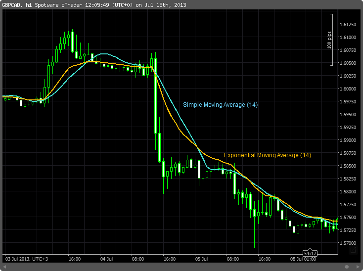
Though I don’t trade stocks, a stock’s price is a great example. When people say to “buy the dip”, they recognize that prices have short-term trends (“the dip”) and long-term trends (a company’s continuing—presumably, anyway—track record of making money and thereby increasing shareholder value). Yet both of these behaviors make up the price. A company’s stock price might fall due to a random string of sells while the company itself makes money over the period at the same rate. If we were long-term traders, then the short-term trends wouldn’t matter to us—they’d be noise, and in this case “high-frequency” noise. We would want to remove them before making our decisions, and that’s where “low-pass filters” would apply. I’m not going to define them more formally, but suffice it to say that moving averages and exponential moving averages happen to fall into this category.
Coincidentally, if we happened to be short-term traders, then the opposite would be true! Long-term trends would be noise, and there are “high-pass filters” for that.
To deal with the noise in the interpolated data, we’ll want to use a low-pass filter. At the time, my choice of a particular one was just a guess: feel free to Google “second-order Butterworth digital filter” or “IIR filters” if you want. Here, just a moving average of the last four frames also suffices.
class MaFilter:
    def __init__(self, n_channels=360, n_samples=4):
        self.samples = np.zeros((n_channels, n_samples))
        self.n_samples = n_samples
        self.i = 0

    def filter(self, x_t):
        self.samples[:, self.i] = x_t
        self.i = (self.i+1)%self.n_samples
        return np.mean(self.samples, axis=1)
Applying this code to our example data yields this
This data is finally a good base to extract motion out of! Now, optical flow has a rich history involving many, many specific end-to-end techniques. “Optical Flow Estimation” by Fleet and Weiss and “Performance of optical flow techniques” by Barron, Fleet, and Beauchemin look to me like very comprehensive descriptions of the older ones. However, since those texts were about applying optical flow on video, let’s work out the same reasoning on our RPLIDAR data. We can let $r(\theta, t)$ be the distance from the RPLIDAR at angle $\theta$ and time $t$. (It’s worth noting here that a single frame here is one-dimensional, but a frame of a video is two-dimensional.) Motion can be expressed as the equality
\[r(\theta, t) = r(\theta+\Delta\theta, t+\Delta t)\]or, in other words, the translation of distances by $\Delta \theta$ over a timespan of duration $\Delta t$. The next step is the “linearization” of this equality: a Taylor series centered at $r(\theta, t)$ replaces the right-hand side, but then we truncate away all terms involving second-order partial derivatives. The approximation we get is
\[r(\theta, t) \approx r(\theta, t) + \frac{\partial r}{\partial \theta} \Delta \theta + \frac{\partial r}{\partial t} \Delta t\]Considering that $\Delta \theta / \Delta t$ is essentially velocity, we can isolate this as the ratio of partial derivatives
\[\frac{\Delta \theta}{\Delta t} \approx - \frac{\partial r / \partial t}{\partial r / \partial \theta}\]This here is the point of divergence from the basic optical flow analysis on two-dimensional frames of video. In the two-dimensional case, the velocity has two components, and we wouldn’t have found an expression for both from a single equation. In general, that’s an underdetermined linear system, also called the “aperture problem” in optical flow texts. Here, the one-dimensional frame means velocity (with a single component) that we can just solve for.
To turn this into a procedure, the partial derivatives can be approximated by the finite differences
\[\frac{\partial r}{\partial t} \approx \frac{r(\theta, t) - r(\theta, t-\Delta t)}{\Delta t}\] \[\frac{\partial r}{\partial \theta} \approx \frac{r(\theta+\Delta \theta, t) - r(\theta-\Delta \theta, t)}{2 \Delta \theta}\]where $t-\Delta t$ means the previous frame, $\theta+\Delta \theta$ means to the next angle in the grid, and $\theta-\Delta \theta$ the previous. $\Delta \theta$ comes from the spacing of the grid, and $\Delta t$ can be measured using Python’s time.time(). Altogether, we have now completely specified one possible velocity estimation procedure. In practice, it gave me a few problems that weren’t just noise.
To be clear, this is the absolute value of the raw velocities times ten. You can see here a couple of issues:
- Small flash-points in the velocity estimation that were consistent enough to beat the low-pass filter
- A hole in the velocity estimate at the center of the moving object
One particular thing I tried that seemingly dealt with both problems is the “Lucas-Kanade method”. Originally, it was devised as the solution to the underdetermined linear system conundrum. On the assumption that neighboring pixels shared the same motion, the equations constructed from these pixels were imported, and this turned an underdetermined system into an overdetermined one with a least-squares solution. Doesn’t the same assumption apply here?
The modified construction is as follows. We can represent the partial derivatives at some $\theta$ and $t$ as $\partial r / \partial \theta \mid_{(\theta, t)}$ and $\partial r / \partial t \mid_{(\theta, t)}$. For some specific $\theta_i$, let’s also consider the 16 angles to its right and the 16 to its left, altogether $\theta_{i-16}, \theta_{i-15}, \dots, \theta_{i+16}$. The partial derivatives (approximated by finite differences) can be taken at these angles and formed into the vectors
\[R_\theta(\theta, t) = \begin{bmatrix} \partial r / \partial \theta \mid_{(\theta_{i-16}, t)} \\ \partial r / \partial \theta \mid_{(\theta_{i-15}, t)} \\ \vdots \\ \partial r / \partial \theta \mid_{(\theta_{i+16}, t)} \end{bmatrix}\] \[R_t(\theta, t) = \begin{bmatrix} \partial r / \partial t \mid_{(\theta_{i-16}, t)} \\ \partial r / \partial t \mid_{(\theta_{i-15}, t)} \\ \vdots \\ \partial r / \partial t \mid_{(\theta_{i+16}, t)} \end{bmatrix}\]What do we do with these vectors? We can start again with the linearization
\[r(\theta, t) \approx r(\theta, t) + \frac{\partial r}{\partial \theta} \Delta \theta + \frac{\partial r}{\partial t} \Delta t\]and manipulate it into the “equation”
\[0 \approx \frac{\partial r}{\partial \theta} \frac{\Delta \theta}{\Delta t} + \frac{\partial r}{\partial t}\]which we can extend with our vectors under the shared motion assumption
\[0 \approx R_\theta \frac{\Delta \theta}{\Delta t} + R_t\]where $R_\theta$ and $R_t$ are just shorthand here for $R_\theta(\theta, t)$ and $R_t(\theta, t)$. Though this vector equation usually doesn’t have a solution, it takes the classic form of “minimize $Ax-b$”. The solution to “minimize $Ax-b$” is $x = (A^\intercal A)^{-1} A^\intercal b$, or in our case
\[\frac{\Delta \theta}{\Delta t} \approx (R_\theta^\intercal R_\theta)^{-1} R_\theta^\intercal R_t\]It is convenient here that $R_\theta$ and $R_t$ are vectors. We can see that $R_\theta^\intercal R_\theta$ is just the square magnitude $\left\Vert R_\theta \right\Vert^2$ and $R_\theta^\intercal R_t$ is just the dot product $R_\theta \cdot R_t$. So, we can just reduce the velocity estimator to just
\[\frac{\Delta \theta}{\Delta t} \approx \frac{R_\theta \cdot R_t}{\left\Vert R_\theta \right\Vert^2}\]Using the following code, we can apply this estimator to our example data and get the following result
class VelocityEstimator:
    def __init__(self, window_size=16):
        self.h_prev = np.zeros(360)
        self.window_size = window_size

    def estimate(self, h, dt):
        dtheta = 2*np.pi/360

        dh_dt = (h-self.h_prev)/dt
        dh_dtheta = (np.roll(h, -1)-np.roll(h, 1))/(2*dtheta)

        dh_dtheta_neighbors = np.empty((360, 2*self.window_size+1), dtype=np.float32)
        dh_dt_neighbors = np.empty((360, 2*self.window_size+1), dtype=np.float32)
        for j in range(2*self.window_size+1):
            shift = j-self.window_size
            dh_dtheta_neighbors[:, j] = np.roll(dh_dtheta, shift)
            dh_dt_neighbors[:, j] = np.roll(dh_dt, shift)

        # calculates all estimated velocities as many dot products
        elementwise_product = np.multiply(dh_dtheta_neighbors, dh_dt_neighbors)
        v_est = -np.sum(elementwise_product, axis=1)/np.sum(dh_dtheta_neighbors**2, axis=1)

        self.h_prev = h
        return v_est
Compared to the results of the other procedure, the hole mostly disappears and the flash-points are suppressed. This signal appears to be so clean that all you could need is a threshold detector (possibly with hysteresis) to find all the directions of motion.
So, that’s the process I used to detect motion using the RPLIDAR. It’s made of a lot of random concepts—perhaps because it was hacked together over a week. So, it might serve more as a demonstration of how these concepts get applied than a whole, proven procedure. I’m sure that there are more effective, simple, or rigorous ways to solve the same problem. Still, this outline hopefully was an interesting read that inspires you to dive deeper into any of the backgrounds it invokes.