Using linear potentiometers for pseudo-logarithmic volume control

Note: This text assumes knowledge of Ohm’s Law, series and parallel resistances, and voltage dividers

Are you trying to control volume in an audio circuit using a potentiometer? Then you should probably want a “logarithmic-taper” potentiometer, also called an “audio-taper” or “A”-taper potentiometer. Those allow you to logarithmically vary the voltage of a signal going through it as you turn.

Potentiometers with A- and B- tapers, shown along with the pseudo-logarithmic technique. By "endolith" via flickr and used under the CC BY-NC-SA 2.0 license

By contrast, ordinary “linear taper”, or “B”-taper, potentiometers vary the voltage linearly—the fraction of the turn you set is exactly the fraction of the original voltage you expect. Then, this voltage drives a speaker at a lower or higher power. However, human hearing has been shown to be logarithmic. For something to sound louder and louder with equal steps, we must dump more and more power into the same sound with every next step.

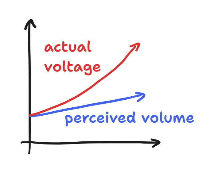
Conversely, we can cut the power by less and less with every step to get something to sound quieter and quieter with equal steps.

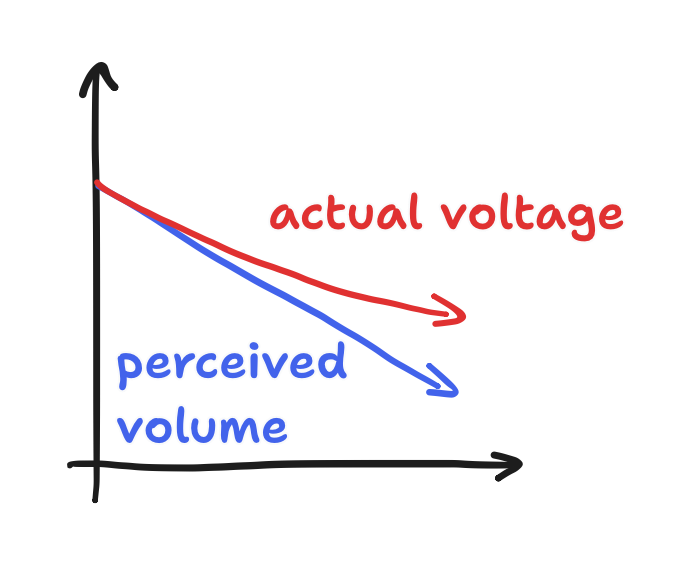
However, linear-taper potentiometers don’t take this human phenomenon into account. As a result, the volume collapses more rapidly as you turn the knob down, and it creeps up more slowly as you turn the knob up. Using a unit called the “decibel”, we can properly plot this behavior on a graph. The “decibel”, formally defined as

$$20 \log_{10} \left( \frac{V}{V_0} \right) \text{dB}$$

where $V / V_0$ is the fraction of the original voltage, is that equal step. Since this fraction is exactly equal to the fraction of the turn for linear potentiometers, we can set this equal to a turn variable $c$ between $0$ and $1$. We can then plot the perceived loudness as $20 \log_{10} c$.

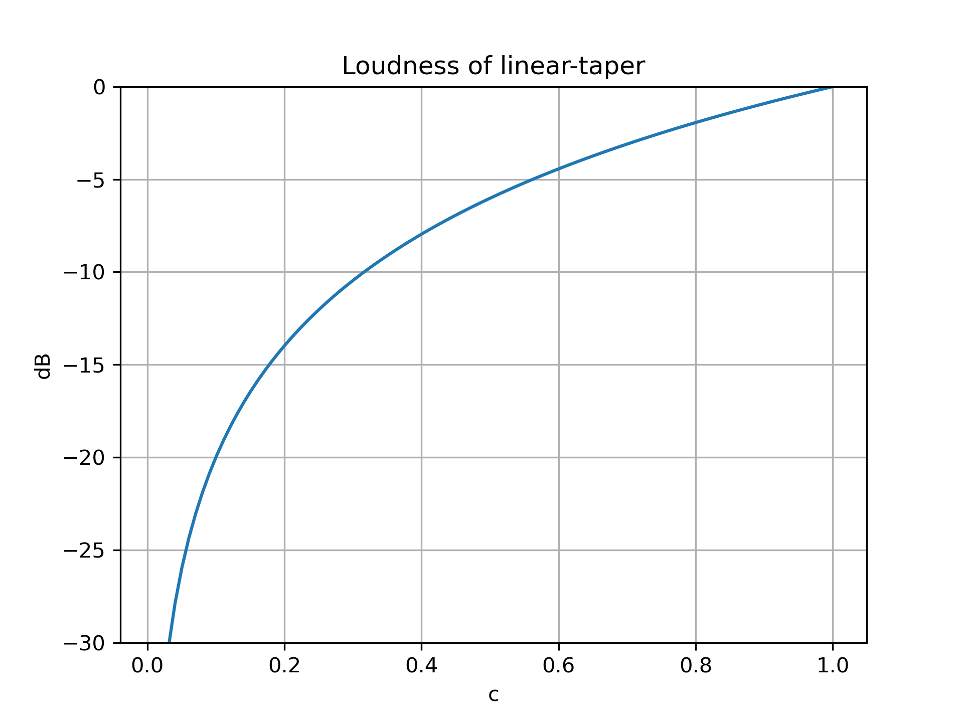
By contrast, logarithmic-taper potentiometers would appear here as a straight line. (In practice, logarithmic-taper potentiometers only approximate the true logarithmic behavior, but they still do a better job than linear-tapers!)

Now, what if we’ve already ordered linear-taper potentiometers but need logarithmic behavior ASAP? You can consider the “loading resistor” technique for a pseudo-logarithmic behavior. This circuit has circulated on the internet long before me, but let’s do a rigorous construction of it to see where and why it works, but also where and why it can fail.

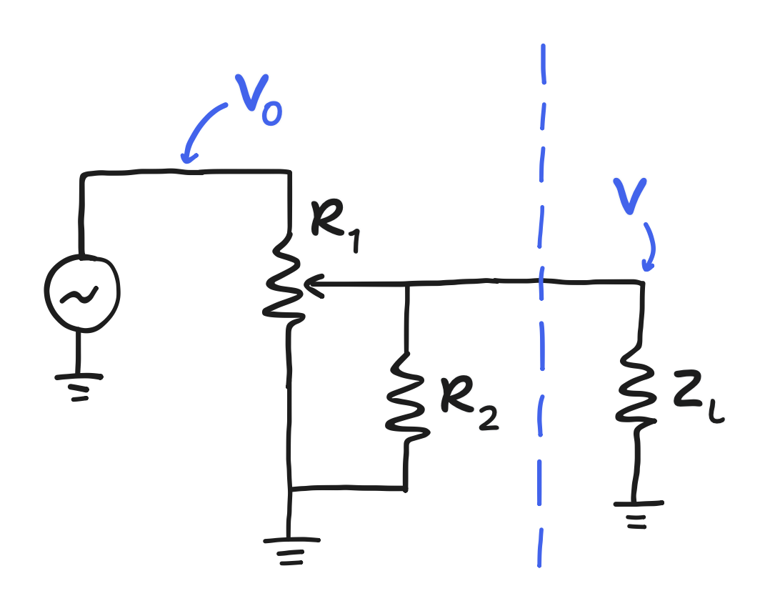
When a potentiometer is used to vary the fraction of the original voltage, it is installed as an adjustable voltage divider.

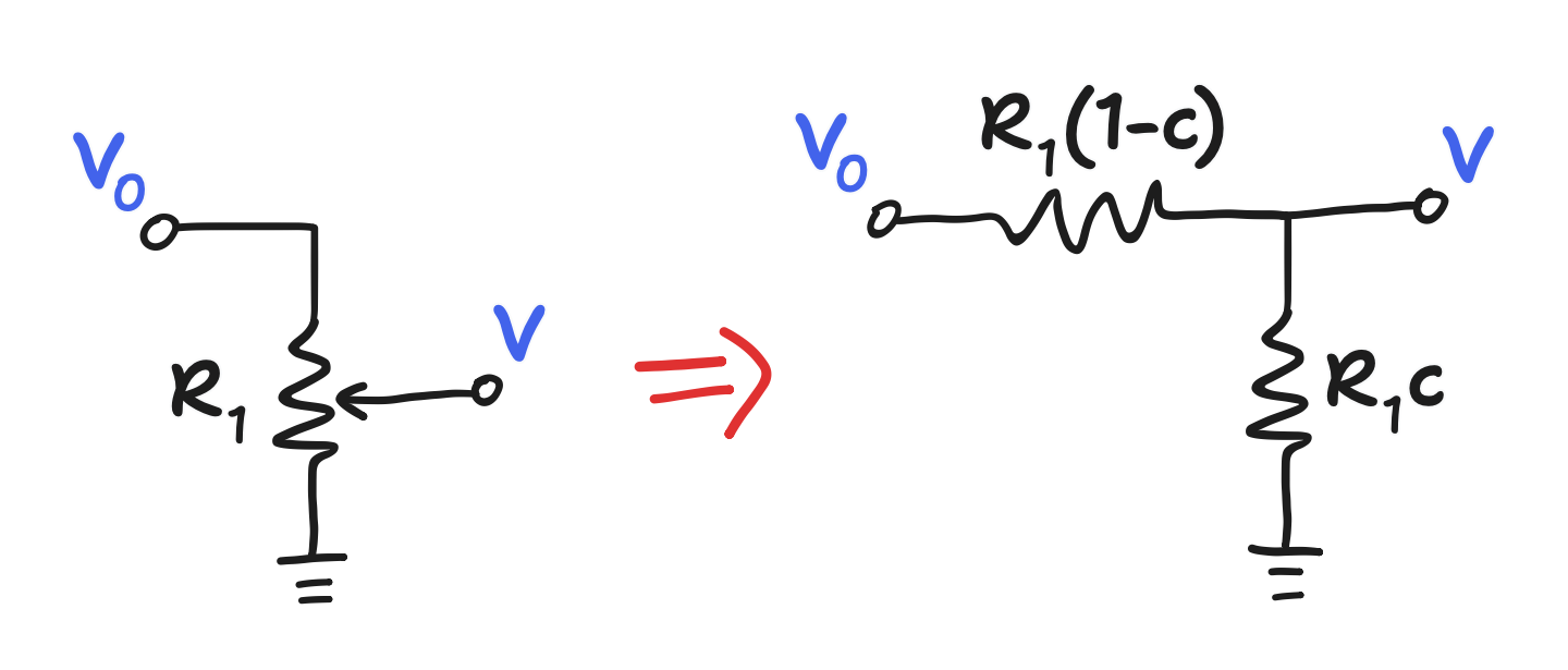
This method works because of the way turning the knob affects the resistances of the upper and lower legs.

$$\begin{align*} \frac{V}{V_0} & = \frac{c R_1}{c R_1 + (1-c) R_1} \\ & = \frac{c R_1}{R_1 + c R_1 - c R_1} \\ & = c \end{align*}$$

On the other hand, the circulating design suggests putting a resistor in parallel with the lower leg

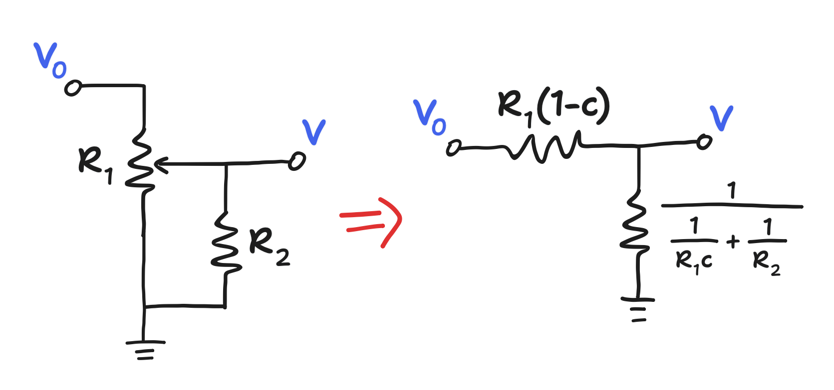
and this gets us a new divider.

$$\begin{align*} \frac{V}{V_0} & = \frac{\frac{1}{\frac{1}{c R_1} + \frac{1}{R_2}}}{\frac{1}{\frac{1}{c R_1} + \frac{1}{R_2}} + (1-c) R_1} \end{align*}$$

This is an intimidating expression! However, sources on the loading resistor design typically mention the ratio between $R_1$ and $R_2$ as the thing to tune. If we let this ratio be the variable $r = R_2/R_1$, the expression can be dramatically simplified.

$$\begin{align*} \frac{V}{V_0} & = \frac{\frac{1}{\frac{1}{c R_1} + \frac{1}{R_2}}}{\frac{1}{\frac{1}{c R_1} + \frac{1}{R_2}} + (1-c) R_1} \\ & \, \, \left\downarrow \frac{1}{\frac{1}{c R_1} + \frac{1}{R_2}} = \frac{c R_1 R_2}{c R_1 + R_2} \right. \\ & = \frac{c R_1 R_2}{c R_1 R_2 + (1-c) R_1 (c R_1 + R_2)} \\ & = \frac{c R_2 / R_1}{c R_2 / R_1 + (1-c)(c + R_2 / R_1)} \\ & \, \downarrow r = R_2 / R_1 \\ & = \frac{c r}{c r + (1-c)(c + r)} \\ & = \frac{cr}{rc + c + r - c^2 -rc} \boxed{ = \frac{cr}{r + c - c^2} } \end{align*}$$

This reduction shows that the behavior of the loading resistor design as you turn the knob—thereby varying $c$—depends only on the ratio $r$. There seem to be many good ratios, but we can take just $r=0.12$ for example. This can be implemented with the potentiometer $R_1$ valued at $100 \text{k}\Omega$ and a loading resistor $R_2$ at $12 \text{k}\Omega$. The behavior in decibels would be

$$20 \log_{10} \left( \frac{0.12 c}{0.12 + c - c^2} \right) \text{dB}$$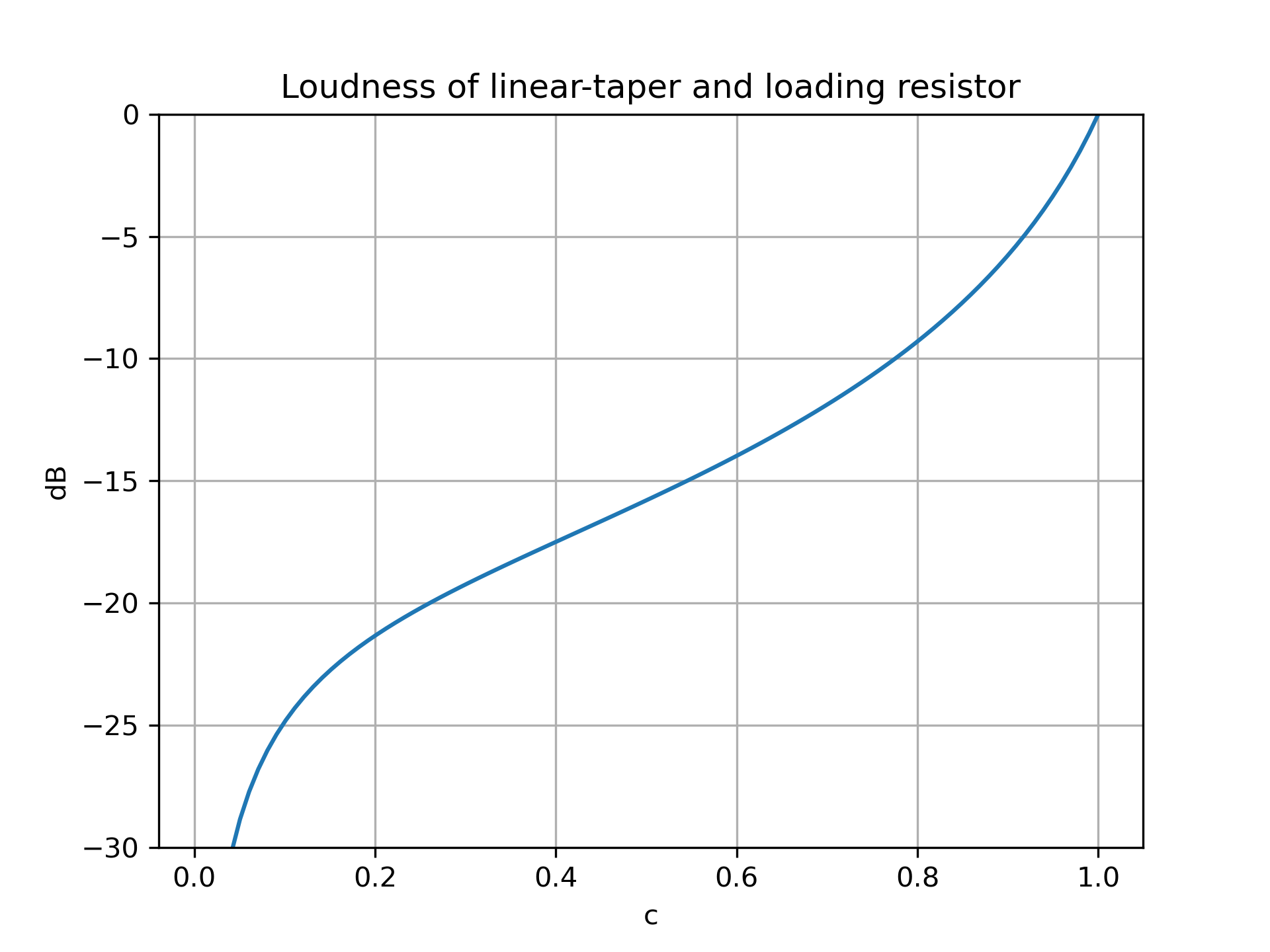

Now, this looks closer to linear! That was a neat result, but the loading resistor method needs to be considered in the bigger picture.

Review: Output impedances and input impedances

You may or may not already know about output impedances and input impedances, so I’ll still cover it here. My understanding of this comes from this excerpt of a Wikipedia article however, so feel free to look there or at other sources as well.

Putting aside all the complexity that goes into designing a good audio amplifier, they’re usually modeled as an “ideal voltage source” chained to an “output impedance”, and if it wasn’t for this output impedance the ideal voltage source could output its set voltage at an infinite amount of current. Instead, as the current drawn increases, the output impedance drops more and more of the set voltage.

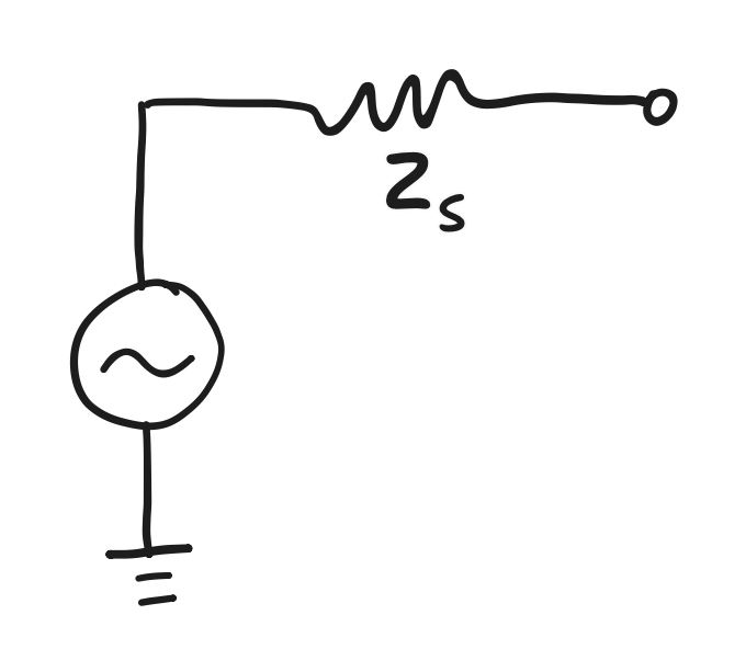
When an amplifier’s spec contains the output impedance, that’s the model invoked. It may be reported as the symbol $Z_s$, and so that will be the symbol used here.

Speakers, headphones, and even the input of an amplifier are usually modeled as a single “input impedance” to represent the fact that they draw current—some more eagerly than others.

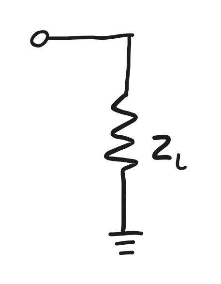
Again, when the specs of these devices include an input impedance, that’s the model invoked. It may be reported as the symbol $Z_L$, and so that will be the symbol used here.

In many diagrams, the bigger picture is not shown, and this usually has no consequence. However, because we’re now holding resistances to specific values, we cannot ignore it: the input and output impedances interfere!

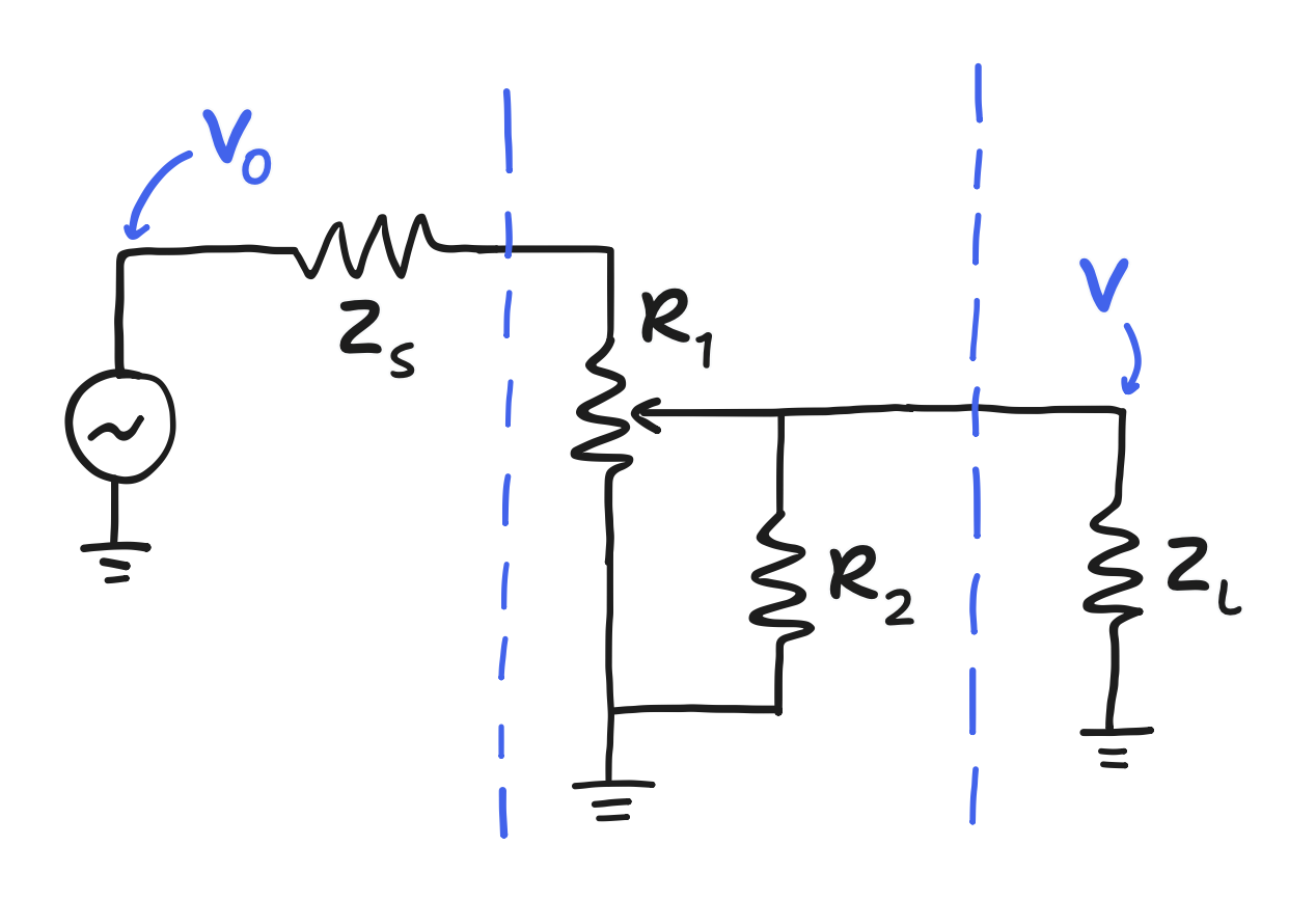
In this scenario, it would technically be possible to calculate exactly what the behavior would be, given the output and input impedances too, then tune $R_1$ and $R_2$ accordingly, but we shouldn’t want to do that. Instead, we can try to claim that the behavior in this bigger picture is a good approximation of the one we originally targeted. To do so, we have to look at the conditions for “neglecting” the input impedance $Z_L$ and the output impedance $Z_S$.

Looking at $Z_S$, we find it in series with the upper leg of the potentiometer $(1-c) R_1$. The condition for “neglecting” that fact is that $Z_S$ is “much smaller than” $(1-c) R_1$. In other words, $Z_S \ll (1-c) R_1$. There’s no solid definition for “much smaller than”, but we can say for now that “much smaller than” means smaller by an order of magnitude, or $Z_S < 10^{-1} \cdot (1-c) R_1$.

Now, $(1-c) R_1$ can actually get arbitrarily small with the right $c$. What we can do about it is give up on getting the approximation right for, say, $c > 0.9$ or the last tenth of the turn in other words. In that case, the condition for neglecting $Z_S$ is now

$$Z_S < 10^{-2} \cdot R_1$$

Going back to the example where $R_1 = 100 \text{k}\Omega$, that means $Z_S < 1 \text{k}\Omega$. If we refer to a Wikipedia excerpt about line-level impedances, we find that line-level output impedances vary from $100 \Omega$ to $600 \Omega$. That means we can neglect $Z_S$ as long as we use a line-level output.

Looking at $Z_L$, we find it parallel with the loading resistor (the lower leg of the potentiometer isn’t part of the problem). The condition for neglecting that fact is that $Z_L$ is “much larger than” $R_2$. Going by “much larger than” meaning larger by an order of magnitude for now, that means

$$Z_L > 10^{1} \cdot R_2$$

Going back to the example where $R_2 = 12 \text{k}\Omega$, that means $Z_L > 120 \text{k}\Omega$. According to the same Wikipedia article, line-level input impedances go from $10 \text{k} \Omega$ and up. So, therefore, we have a problem.

The only universal solution here is to place a unity-gain buffer, but I feel that is outside the scope of this article. Instead, we can talk about what we can do to $R_2$ if we focus on some specific $Z_L$.

If $Z_L$ is on the low end of that “$10 \text{k}\Omega$ and up” range, then we can consider ditching the loading resistor altogether. As a result, $Z_L$ itself is our loading resistor! I saw this approach once in a real inline volume control, and it literally was just a linear-taper $1 \text{k}\Omega$ potentiometer used as a voltage divider. If you used a pair of headphones with an input impedance of $120 \Omega$, then you’d still get a ratio of $r = 0.12$! I suspect that there is some analysis to be done here about damping, but I’m not qualified enough to think about it.

If $Z_L$ is past that low end but not large enough to be neglected, then another possibility is to choose $R_2$ such that $\frac{1}{1/R_2 + 1/Z_L}$ is equal to the $R_2$ you originally wanted.

If $Z_L$ is large enough that it can be neglected after all, then we can plot what the behavior actually looks like in the bigger picture and see that it’s very similar to what we originally targeted!

Curiously, we accepted the possibility of significant error for $c > 0.9$, but this doesn’t materialize. I suspect that there might be an explanation for this revolving around $R_2$. Regardless, at the very least I’m sure that the condition for neglecting $Z_S$ presented will always be sufficient, though it doesn’t appear to be necessary here.

Addendum: “Second-order” Pseudo-logarithmic Volume Control

Notice that the range of volume control for this circuit is 20dB, give or take. There is a class of pseudo-logarithmic volume control circuits that are “second-order” in nature, with a range of around 40dB, though they require an op-amp. Here is the simplest version I’ve found.

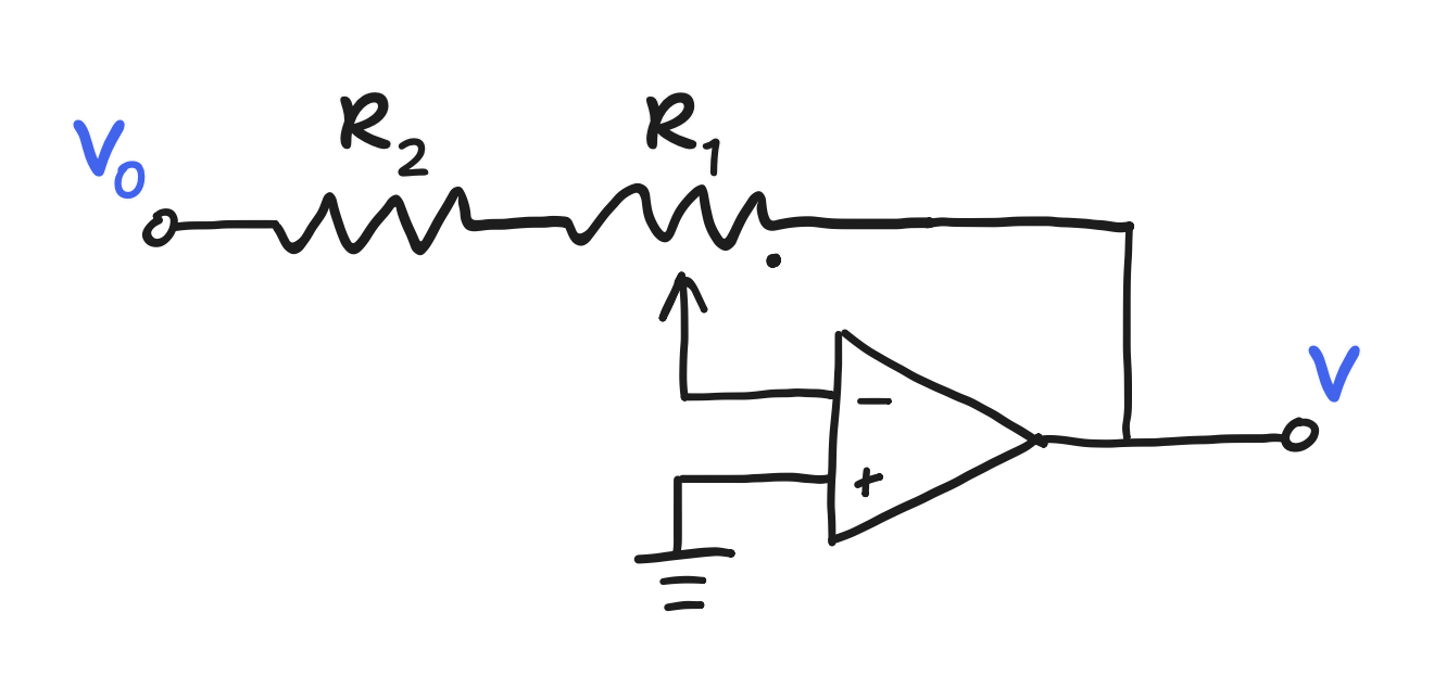
It has a behavior of

$$\frac{V}{V_0} = \frac{-c}{r-c+1}$$

with the decibel plot

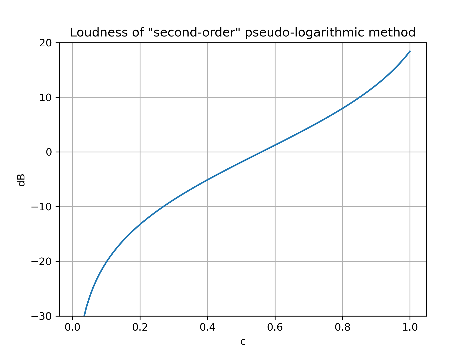
Though, I wouldn’t recommend using this specific example in the real world. If the potentiometer fails, it could break the negative feedback loop, and the op-amp would next go slamming into its rails. I’ve seen some safer “second-order” varieties out there, but I leave designing them as an open question.